3.1.9.1 - Rate Equations

Reading a rate equation

A rate equation describes how concentration affects the rate at a fixed temperature. For example,

The exponents tell you how sensitive the rate is to each concentration. In this specification, the possible orders are limited to 0, 1, and 2.

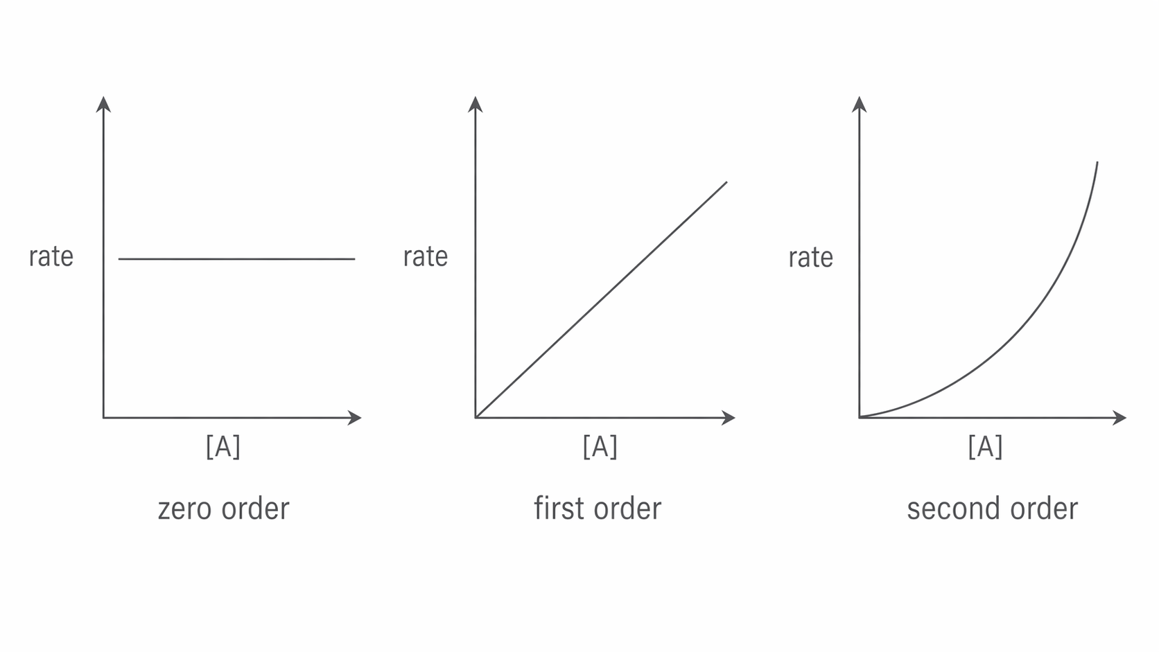
If a reaction is zero order with respect to A, changing $\ce{[A]}$ does not change the rate. If it is first order, doubling $\ce{[A]}$ doubles the rate. If it is second order, doubling $\ce{[A]}$ makes the rate four times larger because the concentration term is squared.

The diagram below compares the shapes of the rate-concentration graphs for zero-order, first-order, and second-order behaviour.

[DIAGRAM: asset_name: 1.9.1 - Rate Equations - Diagram 1; asset_slug: 1.9.1 - Rate Equations - Diagram 1; recommended_method: retained_png; description: Three side-by-side graphs on matching scales, each with rate on the y-axis and [A] on the x-axis. Left graph is a horizontal line labelled zero order. Centre graph is a straight line through the origin labelled first order. Right graph is an upward-curving line from the origin labelled second order.]

The overall order is the sum of the individual orders. So if

the reaction is second order with respect to A, first order with respect to B, and third order overall.

The numbers in the chemical equation do not tell you the order. Orders are found experimentally, not read off from the coefficients in a balanced equation.

Using a rate equation in calculations

Once you know the orders, you can predict how the rate changes when concentrations change. Use the exponents as multipliers on the effect.

Suppose

If $\ce{[A]}$ is doubled while $\ce{[B]}$ stays constant, the rate changes by a factor of $2^{2} = 4$. If $\ce{[B]}$ is halved while $\ce{[A]}$ stays constant, the rate changes by a factor of $1/2$. If both changes happen together, multiply the factors: the new rate is $4 \times 1/2 = 2$ times the original rate.

That last phrase matters. $k$ is constant only if the temperature is constant. It is not the same as the rate itself. If every concentration term in the rate equation equals $1\,\mathrm{mol}\,\mathrm{dm}^{-3}$, using the corresponding concentration and time units, then the numerical value of the rate equals $k$.

You can calculate $k$ by rearranging the rate equation. For example, if

then

Worked example: when $[P] = 0.20\ \mathrm{mol}\,\mathrm{dm}^{-3}$, the rate is $8.0 \times 10^{-4}\ \mathrm{mol}\,\mathrm{dm}^{-3}\,\mathrm{s}^{-1}$.

For this second-order rate constant, the units are:

So $k = 2.0 \times 10^{-2}\,\mathrm{dm}^{3}\, \mathrm{mol}^{-1}\, \mathrm{s}^{-1}$.

For a zero-order reaction $-\mathrm d[A]/\mathrm dt=k$, a straight concentration–time line has gradient $-k$. If $[A]$ falls from $0.080$ to $0.050\,\mathrm{mol\,dm^{-3}}$ in $60\,\mathrm s$, $k=(0.080-0.050)/60=5.0\times10^{-4}\,\mathrm{mol\,dm^{-3}\,s^{-1}}$. Unlike a first- or second-order reactant, its concentration falls by the same amount in each equal time interval while that zero-order behaviour continues. A first-order rate constant has units $\mathrm{s^{-1}}$; for higher orders, derive the units by dividing rate units by all concentration factors.

Why temperature changes k

The temperature dependence of the rate constant is described by the Arrhenius equation.

Here A is the Arrhenius constant, $E_a$ is the activation energy, $R$ is the gas constant, and $T$ is the temperature in kelvin. For this topic, the equation and the value of $R$ are provided when needed, so the important step is using them correctly.