Statistics 5.3 - Hypothesis test for a normal mean | Edexcel A-Level Mathematics

A sample mean below a packet's advertised mass might be ordinary sampling variation, or evidence that the filling machine has shifted. You will test a Normal population mean when its variance is known, given or assumed, using the distribution of the sample mean. Critical values and p-values will lead to the same careful conclusion in context.

Parameter and sample mean

Packets should have population mean mass $500\,\mathrm g$ , but $16$ randomly sampled packets average $497.1\,\mathrm g$ . If individual masses are Normal with standard deviation $6\,\mathrm g$ , is that shortfall convincing evidence that the machine's mean has fallen?

You already know

In $N(\mu,\sigma^2)$ , the second parameter is the variance. A Normal variable is standardised by subtracting its mean and dividing by its standard deviation. A hypothesis test judges evidence assuming the null claim.

The population mean $\mu$ is unknown. The random sample mean $\bar X$ changes from sample to sample; $\bar x=497.1$ is this sample's observed value. Hypotheses concern $\mu$ , not $\bar x$ .

Standard error of the mean

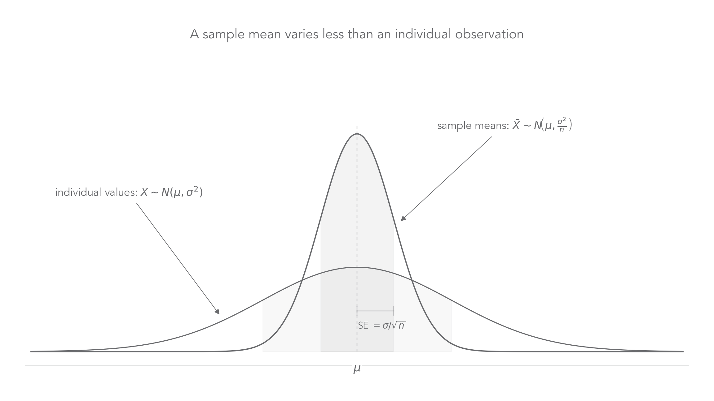
For a random sample of $n$ independent observations from $N(\mu,\sigma^2)$ , the sample mean's standard deviation is $\sigma/\sqrt n$ . This is the standard error: it measures variation between sample means, not variation between individual observations.

Averages are less variable because independent high and low observations partly balance. Here the population is assumed Normal, so the following sample-mean model is exact for every positive sample size; it does not need a large-sample approximation.

Distribution of a Normal sample mean

For a random sample of $n$ independent observations from $N(\mu,\sigma^2)$ ,

\bar X\sim N\left(\mu,\frac{\sigma^2}{n}\right).

The equivalent standardisation is supplied, but this distribution statement is not printed separately.

Not in the formula booklet: learn it.

The diagram shows the common centre and different spreads. The narrower curve describes averages, not a new population of individual packets.

[DIAGRAM: asset_slug: p3_5_3_conduct_a_statistical_hypothesis_test_for_the_mean_of_a_normal_distribution__diagram_01; asset_name: Statistics 5.3 - Hypothesis test for a normal mean - diagram 01; caption: Independent sample averages have less spread than individual values.; description: Two Normal density curves share centre mu, with wider individual distribution and narrower sample-mean distribution, labelled variance sigma squared divided by n and standard error sigma divided by root n.]

Worked example 1: the null sample-mean model

Question. Define the population parameter and set up a test for a fall in the packet mean, using the sample of $16$ and known individual standard deviation $6\,\mathrm g$ .

Plan. Write population hypotheses and divide the individual variance by the sample size.

\begin{aligned} \mu&=\text{population mean packet mass in grams} &&\text{parameter}\\ H_0&:\mu=500\qquad H_1:\mu<500 &&\text{suspected fall}\\ \bar X&\sim N\left(500,\frac{6^2}{16}\right) &&\text{assuming }H_0\\ &=N(500,2.25) &&\text{variance of the mean}\\ \text{standard error}&=\sqrt{2.25}=1.5 &&\text{in grams} \end{aligned}

Why centre the distribution at $500$ , not $497.1$ ? You are judging the observed mean against the null claim.

Answer. Use $\bar X\sim N(500,2.25)$ under $H_0$ , with observed $\bar x=497.1$ .

Check. The sample mean's standard deviation $1.5$ is smaller than the individual standard deviation $6$ .

Change only the sample size from $16$ to $64$ . Four times as many observations halve the standard error, rather than quartering it.

Worked example 2: four times the sample size

Question. Find the null distribution and standard error if the same packet test uses $64$ independent packets.

Plan. Replace $n$ while keeping the population variance and null mean fixed.

\begin{aligned} \bar X&\sim N\left(500,\frac{36}{64}\right) &&\text{same individual variance}\\ &=N(500,0.5625) &&\text{new mean variance}\\ \text{standard error}&=\frac6{\sqrt{64}}=0.75 &&\text{half the old 1.5} \end{aligned}

Why only a halving? Standard deviation uses the square root of the variance, so it changes with $\sqrt n$ .

Answer. The sample mean has null variance $0.5625\,\mathrm{g^2}$ and standard error $0.75\,\mathrm g$ .

Check. $0.75^2=0.5625$ ; the variance is one quarter of $2.25$ .

Keep the random sample mean and its population centre distinct.

Watch out

$H_0:\bar x=500$ is not the population hypothesis. You already know the observed $\bar x$ ; the unknown parameter being tested is $\mu$ .

Use the model in a different population.

Standardising the evidence

The packet sample mean is $2.9\,\mathrm g$ below the null mean. To judge that distance, measure it in standard errors, not in individual packet standard deviations.

Normal mean test statistic

For a random sample from a Normal population with known, given or assumed variance $\sigma^2$ , under $H_0:\mu=\mu_0$ ,

Z=\frac{\bar X-\mu_0}{\sigma/\sqrt n}\sim N(0,1).

In the formula booklet.

Use the population variance specified in the question. If it is $36$ , take $\sigma=6$ . Replacing it by an estimated sample variance would change the procedure being used here.

Worked example 3: standardise the packet evidence

Question. Calculate $z$ for the original packet sample: $\bar x=497.1$ , $n=16$ , $\sigma=6$ , $\mu_0=500$ .

Plan. Find the standard error, then divide the shortfall by it.

\begin{aligned} \frac{\sigma}{\sqrt n}&=\frac6{\sqrt{16}}=1.5 &&\text{standard error}\\ z&=\frac{497.1-500}{1.5} &&\text{distance from the null mean}\\ &=-1.933333\ldots &&\text{standard errors below 500} \end{aligned}

Why divide by $1.5$ , not $6$ ? The evidence is a mean of $16$ packets, whose variation is smaller than one packet's variation.

Answer. $z=-1.93$ to 3 significant figures; retain the unrounded value for probabilities.

Check. The sign is negative because $497.1<500$ .

Change only the observed mean to $498.2\,\mathrm g$ . It is closer to the null mean, so the magnitude should shrink.

Worked example 4: a smaller shortfall

Question. Find $z$ if the same $16$ -packet sample instead has mean $498.2\,\mathrm g$ .

Plan. Keep the standard error and change the numerator.

\begin{aligned} z&=\frac{498.2-500}{1.5} &&\text{same null spread}\\ &=\frac{-1.8}{1.5}=-1.2 &&\text{smaller distance} \end{aligned}

Why keep the denominator? Neither the individual variance nor the sample size has changed.

Answer. $z=-1.2$ .

Check. $|-1.2|<|-1.933333\ldots|$ , agreeing with the smaller shortfall.

A clean standardisation line shows which distribution and variance you used.

Watch out

If $\sigma^2=36$ , the denominator is $6/\sqrt n$ , not $36/\sqrt n$ . Also use $\mu_0$ , not the observed $\bar x$ , as the mean you subtract.

Calculate a positive standardised result next.

Critical regions and p-values

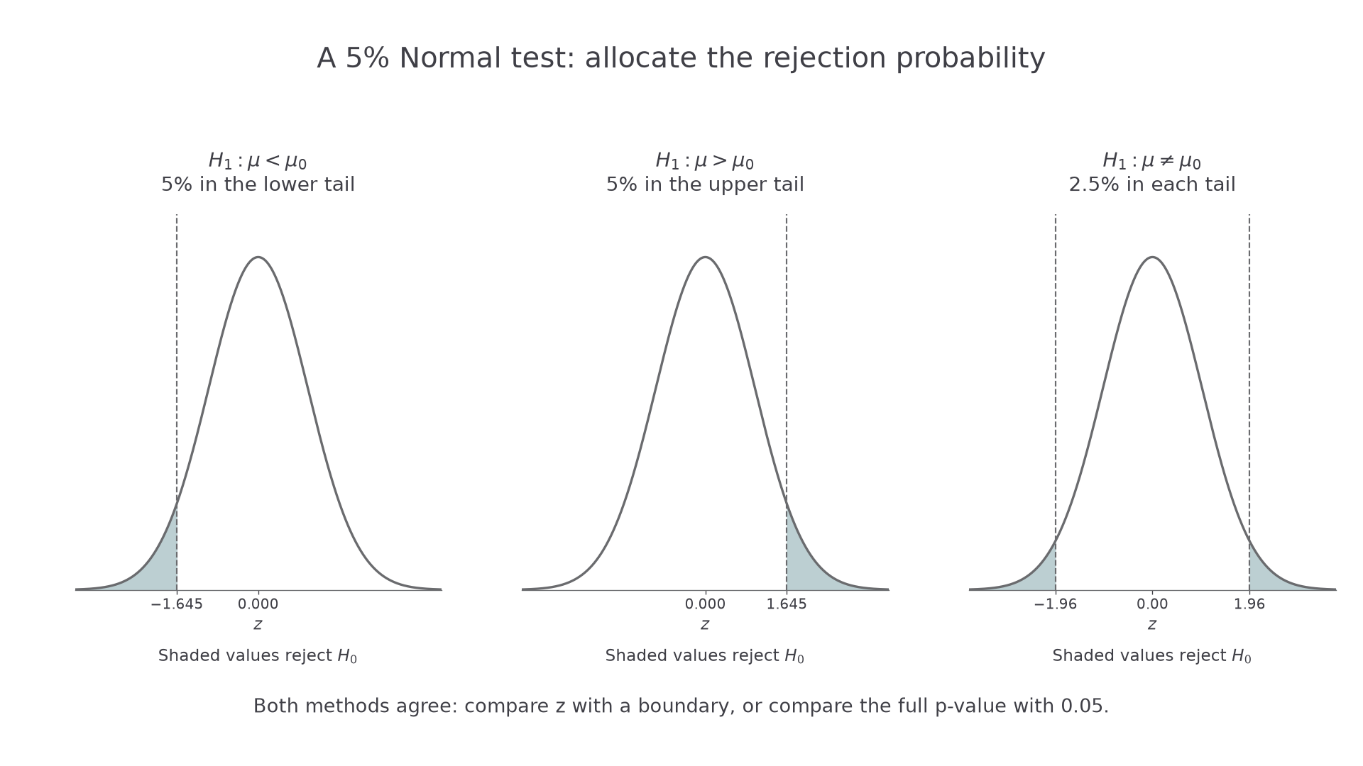
The original packet result is about $1.93$ standard errors below $500$ . Whether it is significant depends on the preselected alternative and level.

The booklet's Normal percentage-point table gives positive $z_\alpha$ satisfying $P(Z>z_\alpha)=\alpha$ . For a lower-tail test use $-z_\alpha$ ; for a two-tailed test share the significance equally between the two tails.

Test at $5\%$	Standard Normal critical region
$H_1:\mu<\mu_0$	$Z<-1.6449$
$H_1:\mu>\mu_0$	$Z>1.6449$
$H_1:\mu\ne\mu_0$	$Z<-1.9600$ or $Z>1.9600$

These rounded table values give the usual boundaries. For a continuous Normal variable, including the exact boundary changes no probability because one exact value has probability zero.

[DIAGRAM: asset_slug: p3_5_3_conduct_a_statistical_hypothesis_test_for_the_mean_of_a_normal_distribution__diagram_02; asset_name: Statistics 5.3 - Hypothesis test for a normal mean - diagram 02; caption: One-tailed and two-tailed tests allocate the same total significance differently.; description: Standard Normal curves show lower and upper 5 percent tails and two 2.5 percent tails with signed numerical boundaries and rejection areas.]

Continue this lesson.

You’re previewing NovaLearn without an account. Create a free account to read the rest.

Create free account

Last Accessed

Pure Mathematics (Papers 1 and 2)

Statistics (Paper 3, Section A)

Mechanics (Paper 3, Section B)

Statistics 5.3 - Hypothesis test for a normal mean

Parameter and sample mean

Standardising the evidence

Critical regions and p-values

Continue this lesson.

Learn faster with Nova