Statistics 2.1 - Single-variable data diagrams | Edexcel A-Level Mathematics

Read histograms, frequency polygons, cumulative frequency diagrams and box plots by identifying what their scales mean. Use them to compare distributions and turn estimated frequencies into probabilities, while keeping track of what grouped data cannot tell you exactly.

What a single-variable diagram shows

Can two equally tall histogram bars represent different numbers of people? Suppose one bar covers times from $4$ to $10$ minutes and another covers $10$ to $14$ minutes. Both have height $5$ . Their widths differ, so their areas differ: $6\times5=30$ and $4\times5=20$ . The taller-looking feature is not always the larger group.

You already know

A rectangle has area $\text{width}\times\text{height}$ . A proportion is a part divided by the whole. These two familiar ideas do most of the work in this lesson.

A diagram compresses a list. That is useful, but the compression hides some information. In Pearson's weather Large Data Set, the $31$ daily mean temperatures at Heathrow in May 2015 fall into the five intervals below. The counts add to $31$ , but the table no longer tells you which date had which temperature.

Temperature, $t$ in ${}^\circ\mathrm C$	$8\le t<10$	$10\le t<12$	$12\le t<14$	$14\le t<16$	$16\le t<20$
Days	1	7	11	10	2

That final class is twice as wide as the others. Drawing its frequency as its height would give it twice the area it deserves. Even a small weather table makes the need for density visible.

Single-variable distribution

A single-variable distribution describes the values of one variable and how often they occur. For example, daily mean temperature at Heathrow is one variable measured on several days. Temperature paired with rainfall is bivariate data instead.

Choose the display for the question you want to answer.

Diagram	Read from it	What it hides or requires care
Histogram	Grouped continuous frequencies from bar areas; distribution shape	Heights are densities when class widths differ
Frequency polygon	Class midpoints plotted against frequencies and joined in order	Points stand for classes, not individual observations
Cumulative frequency diagram	Estimated numbers below values; percentiles	Grouped-data readings depend on interpolation
Box-and-whisker plot	Median, quartiles, spread and separately marked outliers	Detailed shape and peaks are hidden

Key idea

Read the axes and the diagram's conventions before describing the distribution: a height can represent density, frequency or a running total.

Try identifying which display answers a particular question.

Histograms and frequency polygons

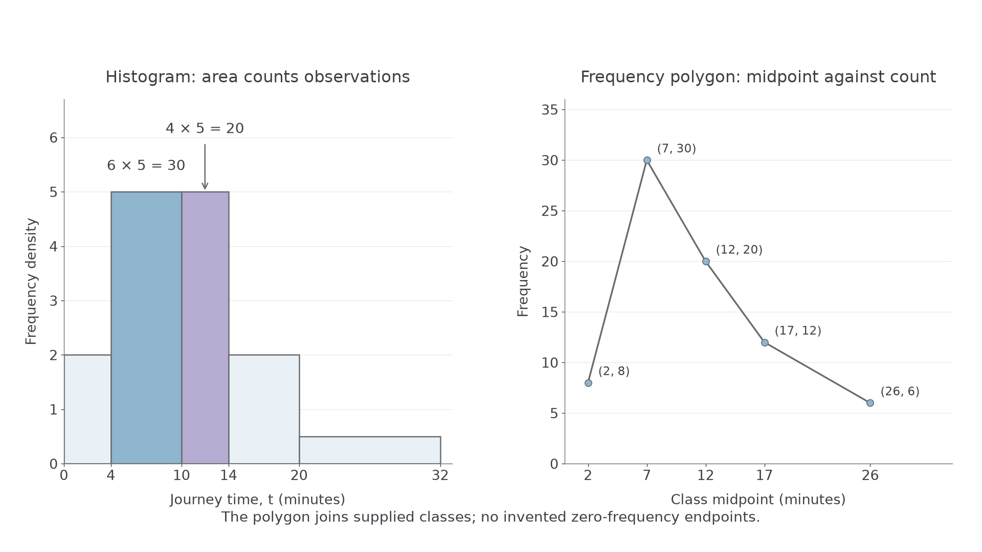
A histogram divides a continuous scale into classes. A bar occupies its whole class interval; adjacent classes meet at their boundaries. Its area represents frequency, so a wider class needs a smaller height for the same frequency.

Histogram area and frequency

For a histogram whose vertical axis is frequency density,

\text{frequency density}=\frac{\text{frequency}}{\text{class width}} \qquad \text{frequency}=\text{class width}\times\text{frequency density}

Use true class boundaries. For measurements rounded to the nearest unit, a class labelled $10$ – $14$ may have boundaries $9.5$ and $14.5$ , not width $4$ . Follow the stated measurement convention.

Not in the formula booklet: learn it.

Here is a sample of $76$ journey times. These are practice data, rather than weather observations.

Time, $t$ in minutes	$0\le t<4$	$4\le t<10$	$10\le t<14$	$14\le t<20$	$20\le t<32$
Frequency	8	30	20	12	6
Frequency density	2	5	5	2	0.5

[DIAGRAM: asset_name: Histogram areas and frequency polygon for journey times; asset_slug: p3_2_1_interpret_single_variable_data_diagrams__diagram_01; caption: Equal histogram heights need not mean equal frequencies; description: Left histogram has class boundaries 0, 4, 10, 14, 20, 32 and densities 2, 5, 5, 2, 0.5. The two bars of height 5 have areas 30 and 20. Right frequency polygon joins class midpoint and frequency points (2, 8), (7, 30), (12, 20), (17, 12), (26, 6).]
Equal histogram heights need not mean equal frequencies

Worked example 1: estimating part of a class

Question. Find the density for $4\le t<10$ , then estimate the number with $6\le t<14$ .

Plan. Divide frequency by width, then add the areas over the requested interval.

\begin{aligned} \text{density}&=\frac{30}{10-4}=5 && \text{use the class width}\\ \text{estimated count}&=(10-6)\times5+20 && \text{part of one bar and a whole bar}\\ &=40 \end{aligned}

Why this step? Splitting the interval at $10$ keeps each area inside one bar. Within a class we assume observations are spread evenly.

Answer. The density is $5$ , and the estimated count is $40$ .

Check. The estimate uses $20$ of the $30$ observations in the first affected class and all $20$ in the next. It lies below their combined frequency $50$ .

Change only the requested interval. Now it crosses a boundary where the density changes.

Worked example 2: crossing unequal densities

Question. Using the same table, estimate the number with $12\le t<18$ .

Plan. Split the interval at $14$ and calculate each rectangle's area.

\begin{aligned} \text{estimated count}&=(14-12)\times5+(18-14)\times2 && \text{use each bar's own height}\\ &=10+8=18 \end{aligned}

Why this step? The density $5$ stops at $14$ ; extending it to $18$ would invent observations.

Answer. About $18$ journeys have times in the interval.

Check. These are half of the $20$ observations in $10\le t<14$ , plus two-thirds of the $12$ in $14\le t<20$ .

A frequency polygon uses the same grouped table differently. Plot class midpoint against class frequency, then join successive points. Here the points are $(2,8)$ , $(7,30)$ , $(12,20)$ , $(17,12)$ and $(26,6)$ . Do not mistake these frequency ordinates for the histogram's density heights. Do not invent zero-frequency endpoints when no such classes are supplied.

Watch out

Wrong: the bar of height $5$ contains $5$ people. Right: the bar from $4$ to $10$ contains $(10-4)\times5=30$ people. If a histogram uses an unlabelled proportional scale, first calibrate area using a known frequency.

Use a new pair of adjacent bars for your own estimate.

Cumulative frequency and box plots

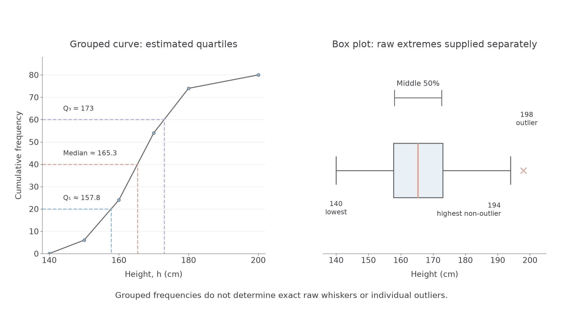
A cumulative frequency diagram answers “How many observations are below this value?” For classes written with an exclusive upper endpoint, add frequencies up to each upper boundary and plot that running total. Start at the lowest boundary with cumulative frequency zero.

For $80$ heights, the running totals below are $6$ , $24$ , $54$ , $74$ and $80$ .

Height, $h$ in $\mathrm{cm}$	$140\le h<150$	$150\le h<160$	$160\le h<170$	$170\le h<180$	$180\le h<200$
Frequency	6	18	30	20	6

Quartiles and a box plot

The quartiles divide an ordered distribution into four parts: $Q_1$ is the lower quartile, $Q_2$ is the median and $Q_3$ is the upper quartile. A box extends from $Q_1$ to $Q_3$ , with a line at the median. When outliers are marked separately, the whiskers end at the most extreme non-outlier observations. Check the stated convention before reading a plot.

For grouped data, read at cumulative frequencies $n/4$ , $n/2$ and $3n/4$ . A straight segment between successive plotted boundaries assumes an even spread within that class. A smooth drawn curve is also an approximation, not recovered raw data.

Reading between cumulative-frequency points

Between $(a,F_a)$ and $(b,F_b)$ , linear interpolation at cumulative frequency $k$ gives

x\approx a+\frac{k-F_a}{F_b-F_a}(b-a)

where $F_a\le k\le F_b$ and $F_b>F_a$ .

Not in the formula booklet: learn it.

The horizontal and vertical guides show the fraction of the class you need.

[DIAGRAM: asset_name: Quartiles from a cumulative frequency graph and a box plot; asset_slug: p3_2_1_interpret_single_variable_data_diagrams__diagram_02; caption: The curve estimates quartiles; the separate box plot needs raw extremes too; description: Left cumulative graph joins (140, 0), (150, 6), (160, 24), (170, 54), (180, 74), (200, 80), with guides at cumulative frequencies 20, 40, 60. Right box plot uses estimated quartiles 157.8, 165.3, 173, and separately supplied raw extremes 140, 194 and outlier 198.]
The curve estimates quartiles

Continue this lesson.

You’re previewing NovaLearn without an account. Create a free account to read the rest.

Create free account

Last Accessed

Pure Mathematics (Papers 1 and 2)

Statistics (Paper 3, Section A)

Mechanics (Paper 3, Section B)

Statistics 2.1 - Single-variable data diagrams

What a single-variable diagram shows

Histograms and frequency polygons

Cumulative frequency and box plots

Continue this lesson.

Learn faster with Nova