Pure 7.1 - Derivatives, tangents and second derivatives | Edexcel A-Level Mathematics

A curve keeps changing its steepness, so how can it have an exact gradient at one point? Build the derivative from nearby chord gradients, prove the first rules, and use first and second derivatives to read a curve's movement and shape.

From straight-line gradient to tangent gradient

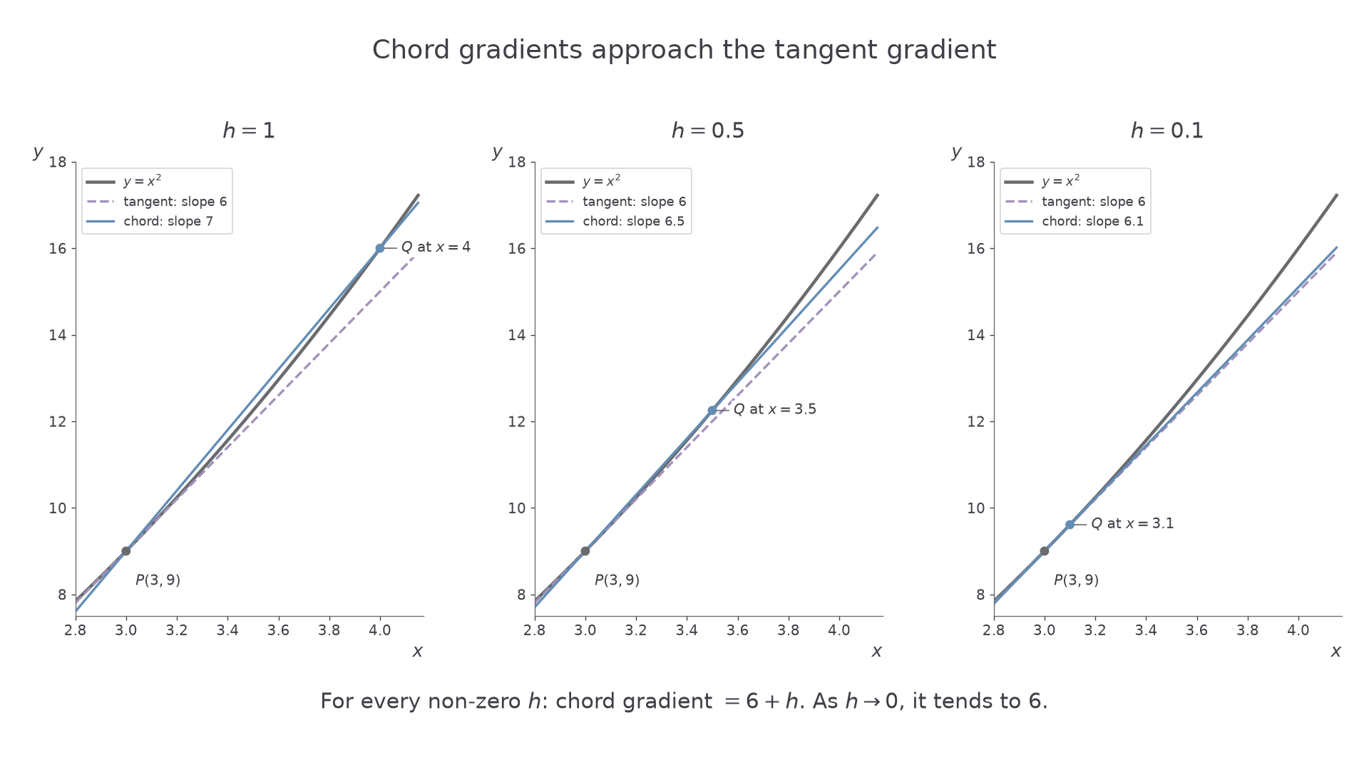
On $y=x^2$ , can you find the exact gradient at $(3,9)$ using two points that are never quite the same? Joining $(3,9)$ to $(4,16)$ gives gradient $7$ . Joining it to $(3.1,9.61)$ gives $6.1$ . The answer seems to be approaching $6$ , but no single finite chord proves that.

You already know

A straight line has gradient $m=(y_2-y_1)/(x_2-x_1)$ , provided $x_2\ne x_1$ . Expanding $(x+h)^2$ gives $x^2+2xh+h^2$ .

The chord joins two points on the curve. A tangent captures its direction locally at one point; it need not meet the curve only once. As the second point approaches the first, the chord gradient can approach one definite value.

[DIAGRAM: asset_slug: p1_7_1_understand_and_use_the_derivative_of_f_x_as_the_gradient_of_the_tangent_and_second_derivative__diagram_01; asset_name: Chords approaching the tangent; caption: Chord gradients approach 6 at P as the second point approaches P; description: On y=x squared, P is (3,9). Chords to x=4, 3.5 and 3.1 have slopes 7, 6.5 and 6.1. The tangent at P has slope 6.]

Derivative

The derivative $f'(a)$ is the finite limiting gradient of chords through $(a,f(a))$ , as the other point approaches it from either side. It is the tangent gradient there and is also written $\left.\frac{\mathrm{d}y}{\mathrm{d}x}\right|_{x=a}$ .

A limit need not be attained by a chord. That is the small but powerful surprise: every non-zero chord width here gives $6+h$ , yet its limiting value is exactly $6$ .

At a sharp corner the two sides can disagree. For $y=|x|$ at zero, the left-hand gradients are $-1$ and the right-hand gradients are $1$ , so there is no derivative there. A finite derivative also requires the function to be defined at the point; at an endpoint only one side may be available.

Key idea

A chord gives an average gradient over an interval; the derivative gives the limiting tangent gradient at one point, when that limit exists.

Use the corner example to separate “a graph exists” from “a derivative exists”.

The derivative as a limit

Give the two points coordinates $(x,f(x))$ and $(x+h,f(x+h))$ . Their horizontal separation is $h$ , so the chord gradient is the change in function value divided by $h$ .

Derivative from first principles

At an interior point where this finite two-sided limit exists,

f'(x)=\lim_{h\to0}\frac{f(x+h)-f(x)}{h}

In the formula booklet.

Keep $h\ne0$ while simplifying. The arrow means “approaches”, not “equals”; putting zero into the original fraction produces the undefined expression $0/0$ .

Worked example 1: the square function

Question. Differentiate $f(x)=x^2$ from first principles and find the gradient at $x=3$ .

Plan. Expand the shifted square, cancel, divide by non-zero $h$ , then take the limit.

\begin{aligned} f'(x)&=\lim_{h\to0}\frac{(x+h)^2-x^2}{h} && \text{definition}\\ &=\lim_{h\to0}\frac{2xh+h^2}{h} && \text{expand and cancel}\\ &=\lim_{h\to0}(2x+h)=2x && \text{divide before the limit} \end{aligned}

Why this step? Cancelling the factor $h$ makes the limiting expression defined at zero.

Answer. $f'(x)=2x$ , so the required gradient is $f'(3)=6$ .

Check. Chord gradients at $x=3$ are $6+h$ ; widths $0.01$ and $-0.01$ give $6.01$ and $5.99$ .

Change one feature: add the linear term $3x$ . Its change is exactly $3h$ , so its contribution to every chord gradient is $3$ .

Worked example 2: adding a linear term

Question. Use first principles to show that $f(x)=x^2+3x$ has derivative $2x+3$ .

Plan. Substitute the entire function at $x+h$ and at $x$ , keeping the subtraction bracket.

\begin{aligned} f'(x)&=\lim_{h\to0}\frac{(x+h)^2+3(x+h)-(x^2+3x)}{h}\\ &=\lim_{h\to0}\frac{2xh+h^2+3h}{h} && \text{collect the change}\\ &=\lim_{h\to0}(2x+h+3)=2x+3 && \text{cancel and take the limit} \end{aligned}

Why this step? Subtracting the whole original function cancels both $x^2$ and $3x$ .

Answer. $f'(x)=2x+3$ , as required.

Check. At $x=2$ , the chord gradient is $7+h$ , approaching $7=2(2)+3$ .

The same subtraction habit matters even when the constant looks harmless.

Watch out

Wrong: cancel $h$ from a sum such as $(x^2+h)/h$ . Cancellation requires a common factor of the whole numerator. Here expansion first creates $h(2x+h+3)$ .

Now alter the coefficient of the linear term and retain the full limit working.

First principles for powers and trigonometric functions

The square proof is the start of a general pattern: in $(x+h)^n-x^n$ , the unshifted term cancels and every remaining term contains $h$ . You need this argument for small positive integer powers, particularly the square and cube.

Worked example 3: the cube

Question. Prove from first principles that $\frac{\mathrm{d}}{\mathrm{d}x}(x^3)=3x^2$ .

Plan. Expand the shifted cube and divide its change by $h$ .

\begin{aligned} f'(x)&=\lim_{h\to0}\frac{(x+h)^3-x^3}{h}\\ &=\lim_{h\to0}\frac{3x^2h+3xh^2+h^3}{h} && \text{binomial expansion}\\ &=\lim_{h\to0}(3x^2+3xh+h^2)=3x^2 && \text{only the constant in }h\text{ remains} \end{aligned}

Why this step? The $h^2$ and $h^3$ terms still matter until division has reduced their powers.

Answer. $\frac{\mathrm{d}}{\mathrm{d}x}(x^3)=3x^2$ .

Check. At $x=2$ , the chord gradient is $12+6h+h^2$ , approaching $12$ .

Change just the multiplier of the same cube; the entire change is doubled.

Worked example 4: a multiple of a cube

Question. Differentiate $f(x)=2x^3$ from first principles.

Plan. Keep the factor $2$ outside the difference quotient.

\begin{aligned} f'(x)&=\lim_{h\to0}\frac{2(x+h)^3-2x^3}{h}\\ &=\lim_{h\to0}2(3x^2+3xh+h^2) && \text{expand and divide}\\ &=6x^2 && \text{take the limit} \end{aligned}

Why this step? Multiplying every height by $2$ doubles every chord gradient.

Answer. $f'(x)=6x^2$ .

Check. At $x=-1$ , the quotient is $6-6h+2h^2$ , approaching $6$ .

Trigonometric proofs use the same definition, but addition formulae replace polynomial expansion. In radians,

\lim_{h\to0}\frac{\sin h}{h}=1,\qquad \lim_{h\to0}\frac{\cos h-1}{h}=0

These two limits are not printed in the booklet. Learn how they are used; a question may supply them. For small positive $h$ , the unit-circle comparison $\sin h<h<\tan h$ squeezes $\sin h/h$ to $1$ ; symmetry gives the negative side. Also $(\cos h-1)/h=-2\sin^2(h/2)/h\to0$ . The addition formulae themselves are supplied.

Worked example 5: sine from first principles

Question. Using the two limits above, show that $\frac{\mathrm{d}}{\mathrm{d}x}(\sin x)=\cos x$ .

Plan. Expand $\sin(x+h)$ , then separate the two known limits.

\begin{aligned} f'(x)&=\lim_{h\to0}\frac{\sin(x+h)-\sin x}{h}\\ &=\lim_{h\to0}\left(\sin x\frac{\cos h-1}{h}+\cos x\frac{\sin h}{h}\right) && \text{addition formula}\\ &=\sin x(0)+\cos x(1)=\cos x && \text{use both limits} \end{aligned}

Why this step? Treat $x$ as fixed while $h$ tends to zero, so $\sin x$ and $\cos x$ are constant multipliers.

Answer. The derivative is $\cos x$ , for radian input.

Check. At zero, the quotient is $\sin h/h\to1=\cos0$ .

Change only the function from sine to cosine. The minus sign in its addition formula changes the final derivative.

Worked example 6: cosine from first principles

Question. Show from first principles that $\frac{\mathrm{d}}{\mathrm{d}x}(\cos x)=-\sin x$ .

Plan. Use $\cos(x+h)=\cos x\cos h-\sin x\sin h$ .

\begin{aligned} f'(x)&=\lim_{h\to0}\frac{\cos(x+h)-\cos x}{h}\\ &=\lim_{h\to0}\left(\cos x\frac{\cos h-1}{h}-\sin x\frac{\sin h}{h}\right) && \text{regroup}\\ &=\cos x(0)-\sin x(1)=-\sin x && \text{take the limits} \end{aligned}

Why this step? The minus sign belongs to the whole sine term and survives the limit.

Answer. The derivative is $-\sin x$ , for radian input.

Check. At $x=\pi/2$ , the cosine graph falls with gradient $-1$ , matching $-\sin(\pi/2)$ .

The derived square, cube, sine and cosine derivative results are not printed in the booklet: learn them. Only the first-principles definition used to establish them is printed there.

Exam tip

If a question requests first principles, show the difference quotient, the expansion or addition formula, and the limiting step. Quoting the final derivative does not establish it.

Use the cosine proof again with a changed constant multiplier.

The derivative as a rate of change

A displacement graph turns gradient into velocity. If $s=t^2+3t$ metres, its derivative $\mathrm{d}s/\mathrm{d}t=2t+3$ has units of metres per second. At $t=4$ , that instantaneous rate is $11\,\mathrm{m\,s^{-1}}$ . The average from zero to four seconds is instead $(28-0)/4=7\,\mathrm{m\,s^{-1}}$ .

Instantaneous rate of change

$\mathrm{d}y/\mathrm{d}x$ measures the limiting change in $y$ per unit change in $x$ . Its units are the units of $y$ divided by the units of $x$ ; it can be negative.

For these polynomial examples, use the derivatives just established and differentiate constant multiples and sums term by term. Their general rules will be developed next lesson; they are not printed in the booklet.

Continue this lesson.

You’re previewing NovaLearn without an account. Create a free account to read the rest.

Create free account

Last Accessed

Pure Mathematics (Papers 1 and 2)

Statistics (Paper 3, Section A)

Mechanics (Paper 3, Section B)

Pure 7.1 - Derivatives, tangents and second derivatives

From straight-line gradient to tangent gradient

The derivative as a limit

First principles for powers and trigonometric functions

The derivative as a rate of change

Continue this lesson.

Learn faster with Nova