Pure 8.8 - Interpreting solutions of differential equations
Solving a differential equation gives a formula; interpreting it tells you what the formula predicts. You will connect initial values, rates, limits and valid domains to a model's quantities and units, including velocity and acceleration, and explain when long-term predictions become unreliable.
The solution as a story
Can a population approach without ever reaching it? Consider , where is measured in thousands and in weeks from the start. At , the denominator is , so there are insects. As time increases, the exponential shrinks and the population rises.
You already know
For , at every finite real , and as . A derivative describes a rate of change, with units of quantity per unit time. These facts are not printed as interpretation rules in the formula booklet.
Reading a solved model means translating its mathematical features back into what is being measured.
Contextual interpretation
A contextual interpretation explains a solution's value, rate, restriction or limiting behaviour using the original quantity and units. A limit is a prediction of the model; it is not automatically an observed value or a value attained at a finite time.
Start with the initial value and the large-time behaviour before attempting a detailed prediction.
Worked example 1: initial and limiting populations
Question. A population is modelled by , for , with in thousands and in weeks. Interpret its initial and limiting values.
Plan. Substitute , then let the exponential tend to zero.
Why multiply the values by ? The formula counts thousands, not individual insects.
Answer. The model predicts insects initially and a population approaching insects in the long term.
Check. The denominator is greater than for every finite , so : the limiting population is approached from below.
Change only the coefficient of the exponential, from to . This changes the initial value while preserving the limit.
Worked example 2: a changed initial population
Question. Interpret the initial and limiting populations for , with the same units and .
Plan. Evaluate the starting denominator and then its limit.
Why is the limit unchanged? The entire exponential term disappears in the limit, whatever its fixed coefficient.
Answer. The population starts at insects and approaches according to the model.
Check. Compared with Worked example 1, the denominator is larger at every finite time, so this population is smaller at each such time but has the same limit.
For a fish model , with in thousands and in months, the corresponding readings are fish initially and a limit of . A change in food supply could change that predicted limit; the formula does not guarantee a permanently fixed environment.
A related differential equation may make the same story visible. For , the solution starts at and approaches , in the chosen population units. The rate is positive between and and becomes smaller near the upper equilibrium.
Watch out
Wrong: “The population is insects after a long time.” The formula measures thousands, and a limit need not be attained. Right: “The model predicts that the population approaches insects.”
Change only the exponential coefficient again.
Reading behaviour from the formula
A solution's form often reveals its behaviour without solving the differential equation again. The expression decreases towards ; the expression keeps growing. Both may be useful models over a suitable interval, but their long-term claims differ.
[DIAGRAM: asset_slug: p1_8_8_interpret_the_solution_of_a_differential_equation_in_context__diagram_01; asset_name: Bounded and unbounded solution models; caption: One solution approaches a finite depth; the other predicts a radius that keeps growing; description: Left panel plots H=0.35+1.15 exp(-0.55t), starting at 1.50 metres, with a horizontal dashed limit at H=0.35 metres. Right panel plots r=(4t+25) to the power two thirds, in centimetres, increasing with decreasing gradient. An annotation explains that a real balloon cannot grow indefinitely, with no invented precise validity cutoff. Each time axis has its own stated units.]
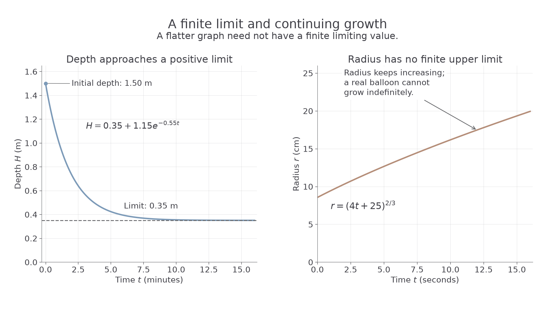
A horizontal asymptote describes the solution's limiting quantity. A gradually flattening curve need not have a finite horizontal asymptote: the balloon's radius grows without bound even though its gradient tends to zero.
Worked example 3: decreasing towards a limit
Question. A reservoir-depth model gives , with in metres, in minutes and . Find its initial depth and limit, and determine whether it is increasing or decreasing.
Plan. Evaluate the endpoints in time and use the derivative's sign.
Why check the derivative? It establishes the direction throughout the interval rather than just comparing two sample depths.
Answer. The depth decreases from towards . In a tank draining through a hole, the limit could represent the hole's height above the base, if that matches the setup.
Check. , so the depth stays above its limit.
Change only the exponential coefficient from to . A reservoir can also approach its settled depth from below.
Worked example 4: increasing towards the same limit
Question. For , in the same units, find the initial depth and limit and determine its direction of change.
Plan. Repeat the initial-value, limit and derivative checks.
Why does the direction reverse? Subtracting a positive term that is shrinking makes the total increase.
Answer. The depth increases from towards , remaining below that limit at every finite time.
Check. For , , so .
A mass model , with in grams and in days, similarly decreases from towards . The same mathematical structure can describe different quantities, but its interpretation must use the actual units.
Watch out
“Gradient tends to zero” does not imply “the quantity tends to a finite value”. For , , yet .
Change only the coefficient in Worked example 4.
Validity and model limits
A formula can be mathematically defined while predicting an impossible physical quantity. For instance, the real cube root of a negative number exists, but a negative radius is impossible. Combine the formula's mathematical domain with the context's restrictions.
Mathematical and contextual restrictions
A mathematical restriction excludes undefined expressions, such as zero denominators or non-positive logarithm arguments. A contextual restriction excludes values that do not represent the situation, such as a negative depth or time before the model starts. The usable model interval must satisfy both, and its assumptions must remain reasonable.
If a differential equation itself becomes undefined at an endpoint, distinguish the limiting predicted quantity from a solution that still satisfies the differential equation there. The examples below concern the supplied solution formula up to the empty state.
Continue this lesson.
You’re previewing NovaLearn without an account. Create a free account to read the rest.
Create free account