Statistics 2.3 - Measures of central tendency and variation | Edexcel A-Level Mathematics

Choose and interpret averages and measures of spread, calculate exact summaries, estimate grouped percentiles, and recover original summaries after coding. Use the supplied standard-deviation formulas with clear units, careful rounding and a reason for the comparison you make.

Centre and spread

Can two sets have the same average but feel completely different? The lists $4,5,6$ and $1,5,9$ both have mean $5$ . The second list is much more spread out. An average alone cannot tell you whether a service is consistent or a machine is reliable.

You already know

The arithmetic mean is the sum divided by the number of values. Order a list before finding its middle, and distinguish a value from the frequency with which it occurs.

[DIAGRAM: asset_name: Same centre and different variation; asset_slug: p3_2_3_interpret_measures_of_central_tendency_and_variation__diagram_01; caption: Identical means can hide four times as much standard deviation; description: Two dot plots on the same horizontal scale show 4, 5, 6 and 1, 5, 9. Both have a marked mean of 5. Their ranges are 2 and 8, and standard deviations using divisor 3 are about 0.816 and 3.27.]

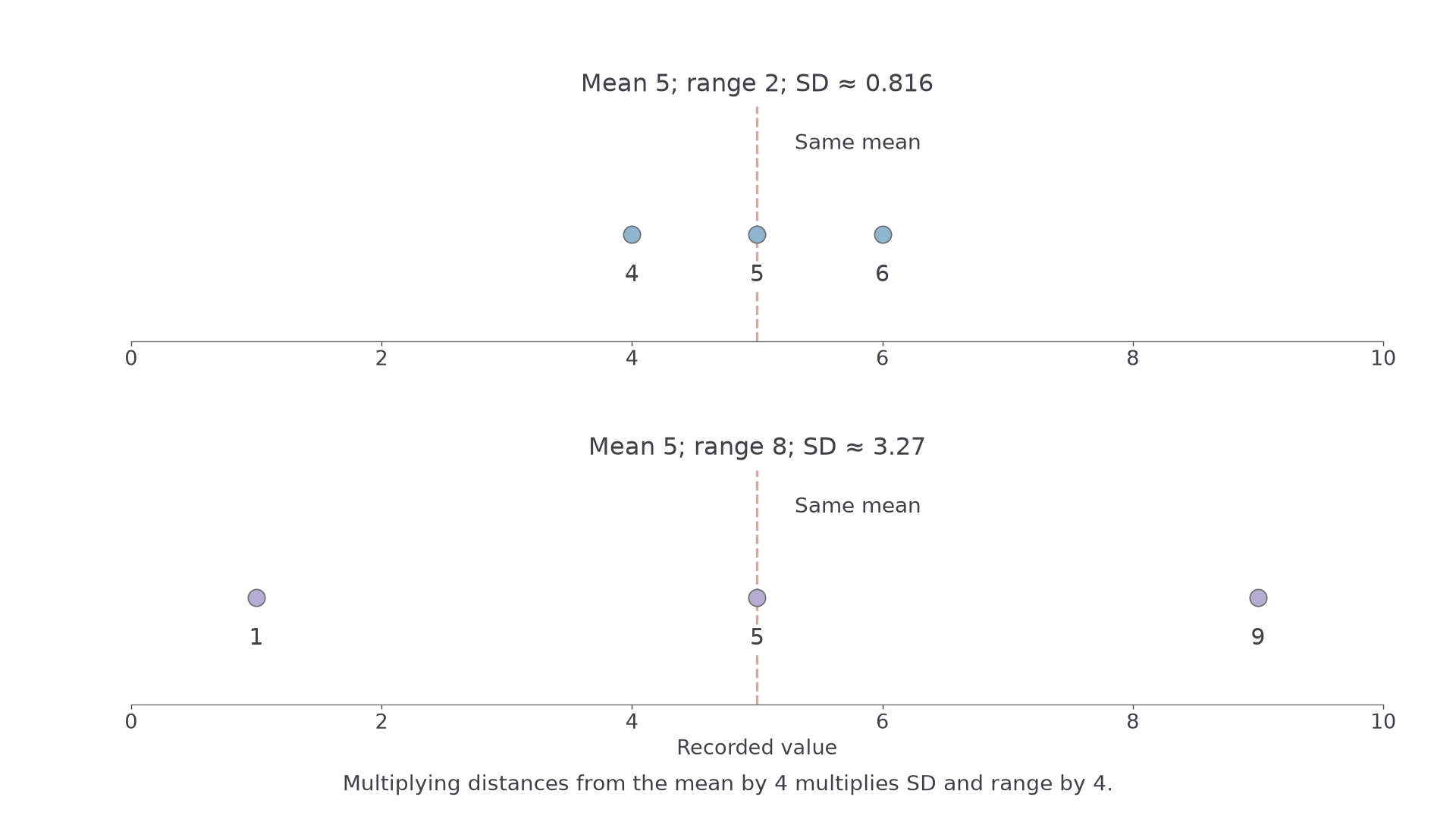
The second list is obtained by multiplying every distance from $5$ by $4$ . Its range and standard deviation are therefore both four times as large. That is a mathematical surprise you can verify without any extra data.

Measures of central tendency

The mean uses every numerical value. The median is the middle value of an ordered list, or the mean of the two middle values. The mode is the most frequent value; there may be several modes or no unique mode. A grouped distribution identifies a modal class rather than an exact modal value.

Extreme values affect the mean because their sizes enter the sum. The median depends on order, so changing an already largest value can leave it unchanged. For skewed data with occasional large values, median and IQR often describe a typical observation more usefully than mean and standard deviation. The mode is useful when the most common category or value is the question.

Measures of variation

The range is the largest value minus the smallest. An interpercentile range is a difference of percentiles, such as $P_{90}-P_{10}$ , measuring the spread of the central $80\%$ . Variance is a mean squared deviation from the mean; standard deviation is its square root.

Standard deviation has the data's units; variance has squared units. A standard deviation of $2\,\mathrm{cm}$ describes variation in lengths, while a variance of $4\,\mathrm{cm^2}$ is its square. Neither is a new average length.

For waiting times, sample A has median $8.1$ , mean $8.3$ , SD $1.4$ minutes; B has median $7.8$ , mean $11.6$ , SD $8.9$ minutes. Their medians are similar, but B has more variation and a mean pulled much further above its median. This is consistent with a long upper tail, although summaries alone do not prove the full shape.

Key idea

Give both centre and spread, chosen for the question and the distribution. A smaller standard deviation means greater consistency, rather than automatically a better outcome for every purpose.

Choose an average that resists one extreme value.

Exact summaries from raw or frequency data

A frequency table can preserve exact recorded values: the frequency tells you how often to count each value. Continuous measurements listed individually also give exact summaries of those recorded measurements, even though the measurements themselves have finite precision.

Mean from a frequency table

For values $x$ with frequencies $f$ ,

n=\sum f \qquad \bar x=\frac{\sum fx}{\sum f}

For a raw list take each frequency as $1$ . The number of distinct rows is not generally the number of observations.

Not in the formula booklet: learn it.

Locate the median by ordered positions, using cumulative frequencies when values repeat.

Worked example 1: an exact frequency table

Question. Late arrivals $x=0,1,2,3,4$ occur with respective frequencies $3,5,6,4,2$ . Find the mean, median, mode and range.

Plan. Find the total and weighted sum, then use cumulative positions for the median.

\begin{aligned} n&=3+5+6+4+2=20 && \text{count all lessons}\\ \sum fx&=0(3)+1(5)+2(6)+3(4)+4(2)=37 && \text{weight by frequency}\\ \bar x&=37/20=1.85 \end{aligned}

The cumulative frequencies are $3,8,14,18,20$ . Positions $10$ and $11$ both contain $2$ , so the median is $2$ . The largest frequency is $6$ , attached to value $2$ . The range is $4-0=4$ .

Why this step? The mode is the value with the largest frequency, rather than the frequency itself.

Answer. Mean $1.85$ , median $2$ , mode $2$ , range $4$ late arrivals.

Check. The weighted mean lies between $0$ and $4$ . It need not be a possible count in one lesson.

Change the presentation from frequencies to a raw list. These are genuine daily mean windspeeds from Heathrow, 1–4 May 2015, in Pearson's Large Data Set.

Worked example 2: a raw weather extract

Question. The windspeeds are $9,9,13,10$ knots. Find the same four summaries.

Plan. Average all four readings, then sort them to find the middle and extremes.

\begin{aligned} \bar x&=\frac{9+9+13+10}{4}=10.25 && \text{four recorded days}\\ \text{ordered list}&:\ 9,9,10,13 && \text{sort before locating the middle}\\ \text{median}&=\frac{9+10}{2}=9.5\\ \text{range}&=13-9=4 \end{aligned}

Why this step? With an even number of readings, the median lies halfway between the two central recorded values.

Answer. Mean $10.25$ knots, median $9.5$ knots, mode $9$ knots and range $4$ knots. Neither the mean nor the median needs to be one of the observations.

Check. The total $41$ equals $4\times10.25$ , and $9$ is the only repeated reading.

For ungrouped quartiles and percentiles, follow a supplied position convention. In the late-arrival list, a rule using positions $5$ and $15$ gives $P_{25}=1$ and $P_{75}=3$ , hence an interpercentile range $2$ . Different software conventions can interpolate differently in small lists; state the requested one.

Watch out

Wrong: divide the late-arrival weighted sum by $5$ , the number of possible values. Right: divide by $20$ , the total frequency. The table's rows compress repeated observations.

Apply the raw-list method to a fresh set of recorded values.

Grouped data and interpolation

Grouping hides where observations lie inside each class. A midpoint mean assumes every observation in a class is at its midpoint; interpolated percentiles assume an even spread within the relevant class. Both are estimates.

Consider these delay times in minutes.

Delay, $x$	$0\le x<10$	$10\le x<20$	$20\le x<30$	$30\le x<40$	$40\le x<60$
Frequency	6	14	20	8	12
Cumulative frequency	6	20	40	48	60

The midpoint mean is $(6(5)+14(15)+20(25)+8(35)+12(50))/60=27$ minutes. For a histogram the modal class is $20\le x<30$ : it has the highest density, $20/10=2$ . The final class is wider, so frequency alone should not be used to compare peak heights.

Grouped percentile interpolation

For percentile $p$ of $n$ observations, use target cumulative frequency $r=pn/100$ . If its class has lower boundary $L$ , width $w$ , frequency $f>0$ and cumulative frequency $c$ before it,

P_p\approx L+\frac{r-c}{f}w

Use boundaries, rather than rounded class labels, and assume an even spread inside the class.

Not in the formula booklet: learn it.

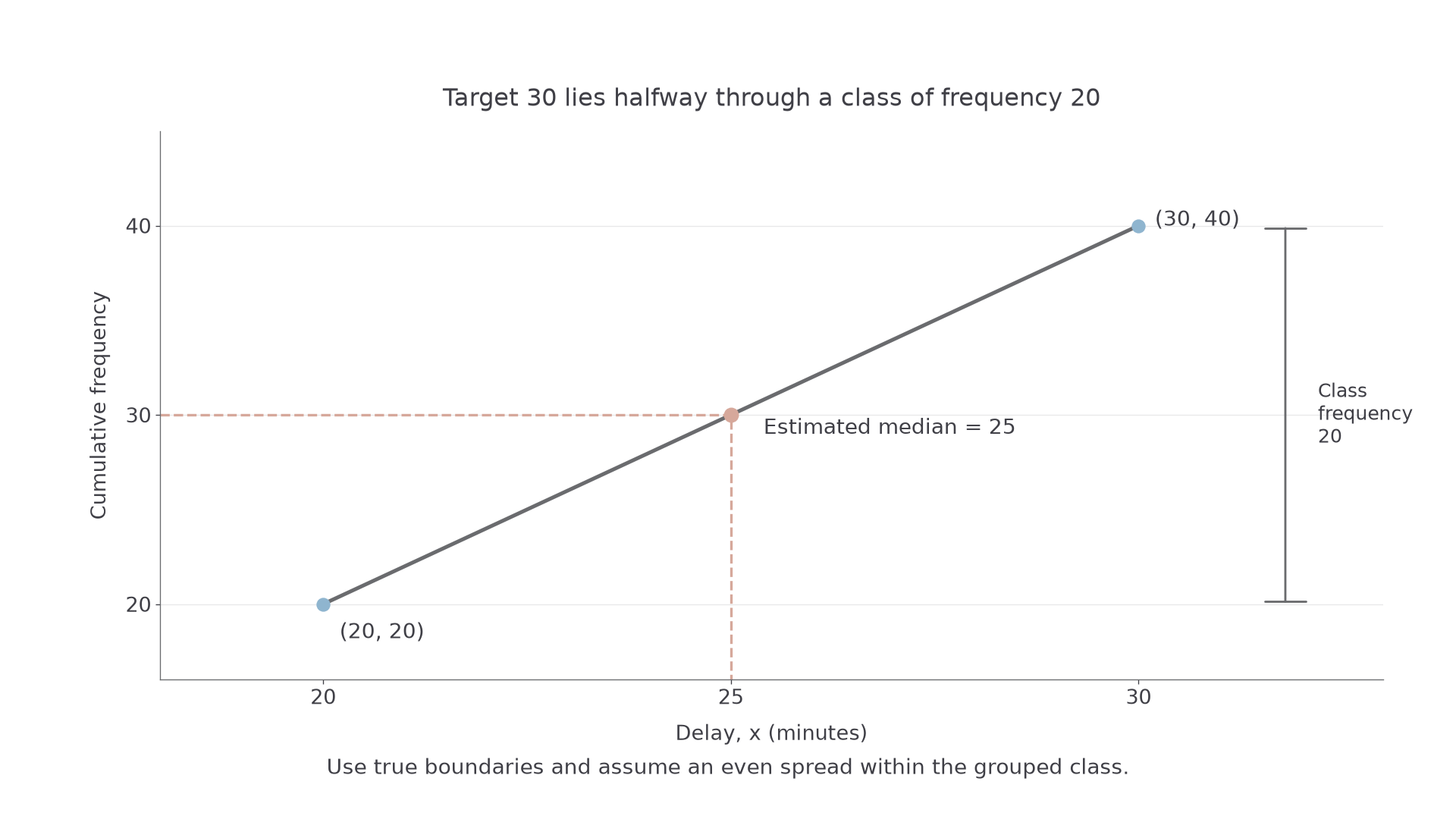
The same fraction appears as a fraction of the horizontal class width.

[DIAGRAM: asset_name: Interpolating within a grouped class; asset_slug: p3_2_3_interpret_measures_of_central_tendency_and_variation__diagram_02; caption: Half the class frequency gives half the class width; description: Cumulative-frequency segment joins (20, 20) and (30, 40). Guides at cumulative frequency 30 meet the segment at x equals 25. Boundaries 20 and 30, class frequency 20 and target 30 are labelled outside the plotted line.]

Worked example 3: estimating a median and percentile range

Question. For the delay table, estimate the median and $P_{90}-P_{10}$ .

Plan. Calculate each target rank and interpolate in its own class.

\begin{aligned} \text{median}&\approx20+\frac{30-20}{20}\times10=25 && r=60/2\\ P_{90}&\approx40+\frac{54-48}{12}\times20=50 && r=0.90(60)\\ P_{10}&\approx0+\frac{6-0}{6}\times10=10 && r=0.10(60) \end{aligned}

Why this step? Percentiles are located by cumulative counts, not by taking a percentage of the largest delay.

Answer. Estimated median $25$ minutes and central $80\%$ spread $50-10=40$ minutes.

Check. The median lies inside $20\le x<30$ ; the target rank for $P_{10}$ is exactly at the first upper boundary.

Change only the pair of percentiles: estimate the spread of the middle half rather than the middle $80\%$ .

Worked example 4: estimating the IQR

Question. Estimate $Q_1$ , $Q_3$ and the IQR for the same table.

Plan. Use target cumulative frequencies $15$ and $45$ .

\begin{aligned} Q_1&\approx10+\frac{15-6}{14}\times10=16.428571\ldots && \text{second class}\\ Q_3&\approx30+\frac{45-40}{8}\times10=36.25 && \text{fourth class}\\ \mathrm{IQR}&\approx36.25-16.428571\ldots=19.821428\ldots \end{aligned}

Why this step? Each percentile may lie in a different class; its width and frequency must come from that class.

Answer. $Q_1\approx16.4$ , $Q_3\approx36.3$ and IQR $\approx19.8$ minutes to $3$ significant figures.

Check. The middle $50\%$ spread is less than the earlier middle $80\%$ spread of $40$ minutes. Unrounded quartiles were subtracted.

The IQR identity itself, $Q_3-Q_1$ , is in the formula booklet; the interpolation process is not. For continuous classes with half-open endpoints, do not add an extra unit to a width. A class $20\le x<30$ has width $10$ .

Exam tip

Write an interpolation expression and call the answer an estimate. Rounding each percentile before subtracting can spoil the final spread.

Estimate a new upper quartile using its own class information.

Continue this lesson.

You’re previewing NovaLearn without an account. Create a free account to read the rest.

Create free account

Last Accessed

Pure Mathematics (Papers 1 and 2)

Statistics (Paper 3, Section A)

Mechanics (Paper 3, Section B)

Statistics 2.3 - Measures of central tendency and variation

Centre and spread

Exact summaries from raw or frequency data

Grouped data and interpolation

Continue this lesson.

Learn faster with Nova