Statistics 2.2 - Scatter diagrams and regression lines
Read paired data, describe its relationship and interpret a supplied regression line in context. Decide when a prediction is defensible, distinguish association from cause, and use logarithms to recover a curved model from a transformed straight line.
Bivariate data and variables
If windy days have stronger gusts, has a scatter diagram proved that the daily mean causes the gust? Start with real pairs. In Pearson's Large Data Set, Heathrow on 1 May 2015 has daily mean windspeed knots and maximum gust knots. On 5 May the pair is . Pairing the measurements preserves information that two separate lists would lose.
You already know
A point records a horizontal coordinate followed by a vertical coordinate. Substituting into gives the vertical value predicted at a chosen horizontal value.
The first seven May 2015 pairs are shown below. Each column describes the same day in both rows; sorting each row independently would destroy the pairing.
| Date in May 2015 | 1 | 2 | 3 | 4 | 5 | 6 | 7 |
|---|---|---|---|---|---|---|---|
| Mean windspeed, knots | 9 | 9 | 13 | 10 | 19 | 18 | 10 |
| Maximum gust, knots | 21 | 21 | 33 | 24 | 43 | 39 | 25 |
Bivariate data and variable roles
Bivariate data records paired values of two variables for each observation. The explanatory or independent variable is used to predict the response or dependent variable. Usually plot the explanatory variable horizontally and the response vertically. These roles describe the proposed prediction; they do not establish causation.
To predict maximum gust from mean windspeed, use mean windspeed horizontally. To investigate revision hours as a predictor of test score , plot . The letters can change; the roles matter. Two rainfall values from unrelated days do not become a meaningful pair merely because they are written next to each other.
Key idea
One point represents one paired observation. Choose axes from the prediction being investigated, rather than from which letter happens to be called .
Use the stated purpose to identify the roles.
Correlation patterns
Correlation describes how paired values vary together. First describe the direction, then how tightly the points follow a straight-line pattern.
| Description | What the scatter shows |
|---|---|
| Positive correlation | Larger explanatory values tend to accompany larger responses |
| Negative correlation | Larger explanatory values tend to accompany smaller responses |
| Zero linear correlation | No overall straight-line trend; a curved relationship can still exist |
| Strong linear correlation | Points lie close to a straight-line pattern |
| Weak linear correlation | Points are more dispersed about that pattern |
[DIAGRAM: asset_name: Correlation and distinct groups; asset_slug: p3_2_2_interpret_scatter_diagrams_and_regression_lines_in_bivariate_data__diagram_01; caption: Direction, strength and separate groups need separate attention; description: Four scatter panels show strong positive correlation, weak negative correlation, a symmetric curved pattern with no linear trend, and two separated groups. In the last panel group A contains (1, 8), (2, 7), (3, 6) and group B contains (7, 18), (8, 17), (9, 16); both decrease within their own group although the combined data rise overall.]
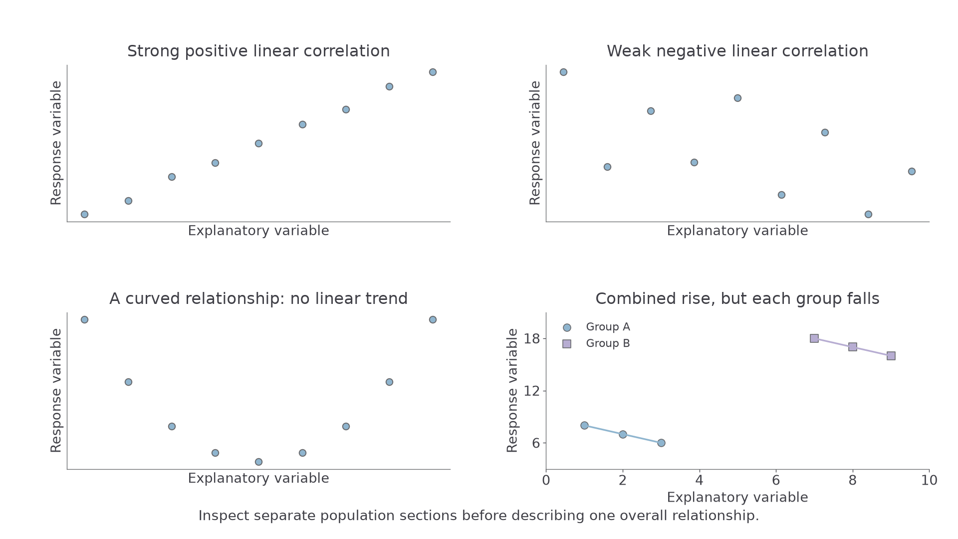
The last panel contains a useful surprise: each group slopes downwards, but the combined cloud slopes upwards. Its six pairs are , , , , and . Moving from the lower group to the upper group creates the overall positive association. One line for the whole population hides its two sections.
Linear correlation
Linear correlation describes the direction and strength of a straight-line association. “No linear correlation” is not the same as “no relationship”: points following a U-shaped curve provide a counterexample.
If age is plotted against reaction time and points rise closely along a line, describe strong positive correlation: greater ages tend to accompany longer reaction times. If a temperature–bottle-sales cloud rises but is widely scattered, describe weak positive correlation. Neither statement says every individual pair follows the trend exactly.
For data containing distinct stations, age groups or other sections, describe both the overall pattern and any different within-group patterns. Marker shapes or colours can reveal distinctions that an unlabelled cloud conceals.
Key idea
Check for curves and separate groups before summarising the whole scatter with one positive or negative trend.
The shape of the cloud matters more than whether its highest point is high.
Interpreting given regression lines
A supplied regression line summarises a linear relationship by predicting the response from the explanatory variable. Interpret the equation and use it; you do not need to derive a least-squares line from raw data here.
Regression line of response on explanatory variable
In a line , is the predicted response at explanatory value . The gradient is the predicted change in for a one-unit increase in . The intercept is the predicted response at , which may lie outside the observations.
A line predicts a typical response, not the exact result of every observation. Its gradient has units of response divided by explanatory variable. Thus , with cost in pounds and distance in kilometres, predicts an extra per extra kilometre. It does not predict that every taxi charges this rate.
Worked example 1: interpreting a decreasing response
Question. A supplied model for a bird's height metres after seconds is . Interpret its gradient and predict the height at .
Plan. Read the coefficient of time as a rate, then substitute the time.
Why this step? The negative sign describes decreasing height; the magnitude and units say how much decrease is predicted per second.
Answer. Each additional second predicts a decrease of in height. The predicted height after seconds is .
Check. In seconds the predicted fall is , less than the initial .
Change only the gradient. The intercept and requested time stay the same, so you can see exactly which prediction changes.
Worked example 2: comparing a changed gradient
Question. Another supplied line is . Interpret its gradient and predict at .
Plan. Give a contextual rate and substitute as before.
Why this step? A more negative gradient means a larger fall per second, rather than a smaller initial height.
Answer. Height is predicted to decrease by each second; at seconds it is .
Check. The gradient differs by per second, so the predictions differ by .
The intercept predicts height at time zero. In a different context, zero may have no sensible interpretation: a regression using adult heights cannot justify a prediction for a person of zero height.
Exam tip
An interpretation such as “negative correlation” does not interpret a gradient fully. Give the direction, amount, variables and rate units, for example a fall of per second.
Read a fresh line in the same way.
Interpolation, extrapolation, and model fit
A correct substitution can still give an unreliable prediction. You need the observed explanatory range and the scatter's shape as well as the line.
Interpolation and extrapolation
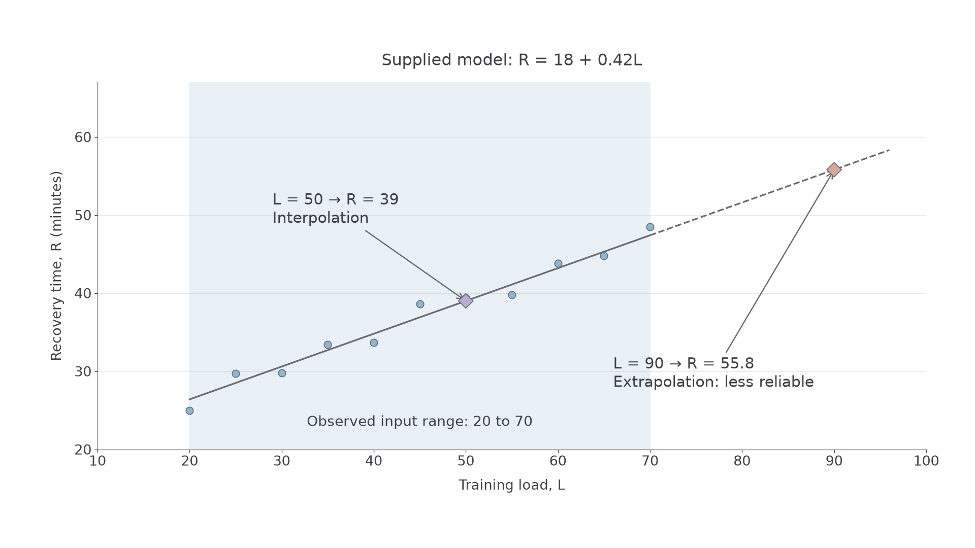
Interpolation predicts within the observed range of explanatory values. Extrapolation predicts outside that range. For observations with , using is interpolation and using is extrapolation.
The relationship may bend, level off or cease to apply outside the observed range. Even interpolation can be poor when the scatter is curved, widely dispersed or made of distinct groups.
[DIAGRAM: asset_name: Observed range and predictions; asset_slug: p3_2_2_interpret_scatter_diagrams_and_regression_lines_in_bivariate_data__diagram_02; caption: A line extends beyond the evidence used to fit it; description: Recovery-time practice data cover training load 20 to 70 around R equals 18 plus 0.42L. Solid line within the observed range and dashed extension to 95; prediction at L equals 50 is 39 and interpolation, while L equals 90 gives 55.8 and extrapolation.]
Continue this lesson.
You’re previewing NovaLearn without an account. Create a free account to read the rest.
Create free account