Pure 6.7 - Exponential growth and decay in modelling | Edexcel A-Level Mathematics

Build exponential models from observations, interpret their constants and use logarithms to find when a threshold is reached. You will distinguish continuous rates from percentage changes over a whole year, then check whether the model's long-term predictions fit the context.

The model and its parameters

Algae cells increase from $3.2$ thousand to $5.0$ thousand in $6$ days. If a container can support about $20$ thousand, how long could exponential growth continue? A constant six-day multiplier would predict $5.0(5.0/3.2)=7.8125$ thousand after another $6$ days. Repeated multipliers soon challenge a limited container; we will find when the model reaches its stated limit.

You already know

An exponential function stays positive. Logarithms undo an unknown exponent, and $e^{u+v}=e^ue^v$ . The gradient of $e^{kt}$ is $ke^{kt}$ , so an exponential can describe a rate proportional to the current amount.

A model is a mathematical description chosen for a purpose. The contexts and values in the calculations below are mathematical modelling scenarios; their predictions need checking against observations before being used in practice.

Initial value

The initial value is the model's value when its time variable is $t=0$ . If $t$ counts years after a specified date, “initial” refers to that date, even when the earliest observation occurs later.

The initial amount fixes the starting height. A second constant determines the repeated multiplier.

Exponential growth and decay

For a positive quantity and a constant continuous proportional rate,

Q(t)=Ae^{kt},\qquad A>0

Here $Q(0)=A$ , and over an interval of length $h$ ,

\frac{Q(t+h)}{Q(t)}=e^{kh}

Growth has $k>0$ , decay has $k<0$ , and $k=0$ gives a constant quantity. If $t$ is in hours, $k$ has units $\mathrm{h}^{-1}$ , so $kt$ has no units.

Not in the formula booklet: learn it.

The ratio follows by cancelling $A$ and subtracting the exponents. Also, $\dfrac{\mathrm{d}Q}{\mathrm{d}t}=kAe^{kt}=kQ$ : the continuous rate of change is proportional to the amount currently present. The exponential-gradient rule is recall knowledge and is not printed in the formula booklet.

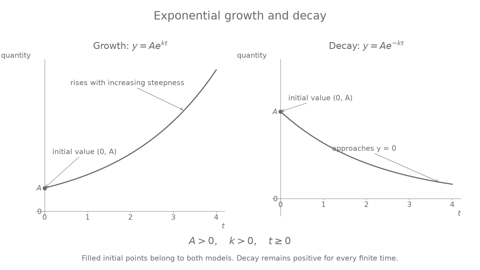
[DIAGRAM: asset_name: Exponential growth and decay; asset_slug: p1_6_7_understand_and_use_exponential_growth_and_decay_in_modelling__diagram_01; caption: Growth increases without bound; decay remains positive and approaches zero; description: Two panels compare Ae to the kt with Ae to the minus kt for positive A and positive k. Both start at A when t=0. In the decay panel, the minus sign gives a negative continuous proportional rate.]

Worked example 1: interpret a decaying amount

Question. A chemical mass in grams is modelled by $N(t)=180e^{-0.07t}$ , with $t$ in days. State its initial mass and find its daily multiplier and daily percentage decrease.

Plan. Put $t=0$ for the initial value and use $e^k$ for the one-day multiplier.

\begin{aligned} N(0)&=180e^0=180 &&\text{initial time}\\ \frac{N(t+1)}{N(t)}&=e^{-0.07}=0.932393\ldots &&\text{one-day interval}\\ 100(1-e^{-0.07})&=6.76061\ldots &&\text{percentage lost per day} \end{aligned}

Why this step? The coefficient $-0.07$ is a continuous rate, so the daily decrease is not exactly $7\%$ .

Answer. Initially $180\,\mathrm{g}$ ; daily multiplier $0.932$ ; decrease $6.76\%$ per day, to $3$ significant figures.

Check. $180e^{-0.07}\approx167.831\,\mathrm{g}$ , a positive amount below $180\,\mathrm{g}$ .

Worked example 2 changes only the sign of the exponent. The initial mass is unchanged, but the multiplier now exceeds $1$ .

Worked example 2: reverse decay to growth

Question. Instead let $N(t)=180e^{0.07t}$ , with the same units. Find the initial mass, daily multiplier and daily percentage increase.

Plan. Use the same substitutions, with a positive continuous rate.

\begin{aligned} N(0)&=180 &&\text{the starting value is unchanged}\\ \frac{N(t+1)}{N(t)}&=e^{0.07}=1.072508\ldots &&\text{daily multiplier}\\ 100(e^{0.07}-1)&=7.25081\ldots &&\text{percentage gained per day} \end{aligned}

Why this step? A percentage increase is the multiplier minus $1$ , multiplied by $100$ .

Answer. Initially $180\,\mathrm{g}$ ; daily multiplier $1.07$ and daily increase $7.25\%$ , to $3$ significant figures.

Check. The unrounded growth and decay multipliers multiply to $e^{0.07}e^{-0.07}=1$ . Their percentage changes need not be equal.

Always attach the time interval to a multiplier or percentage. “The population rises by $0.12$ ” does not explain a continuous coefficient of $0.12\,\mathrm{h}^{-1}$ .

Watch out

Wrong: $Ae^{0.12t}$ means $12\%$ growth each hour. Right: when $t$ is in hours, the hourly multiplier is $e^{0.12}$ , so the hourly increase is $100(e^{0.12}-1)\%$ .

Identify the starting value and the time unit in the next model before calculating.

Finding constants from data

Each observation gives an equation in $A,k$ . An observation at $t=0$ gives $A$ immediately. If neither observation is initial, divide the equations so that $A$ cancels.

Recover a constant continuous rate

If $Q_1=Ae^{kt_1}$ and $Q_2=Ae^{kt_2}$ , where $Q_1,Q_2>0$ and $t_2\ne t_1$ , then

\frac{Q_2}{Q_1}=e^{k(t_2-t_1)},\qquad k=\frac{\ln(Q_2/Q_1)}{t_2-t_1}

Use the same units for both times. Recover $A$ from $A=Q_1e^{-kt_1}$ .

Not in the formula booklet: learn it.

The denominator is elapsed time, not the later time on its own. Keep the unrounded logarithmic value of $k$ for later predictions, even when you display a rounded model.

Worked example 3: an initial observation

Question. A drug concentration in $\mathrm{mg\,L^{-1}}$ follows $C(t)=Ae^{kt}$ , with $t$ in hours. Initially $C=72$ ; after $4$ hours, $C=43$ . Find the model, giving $k$ to $3$ significant figures.

Plan. Use the initial value for $A$ , then solve one exponential equation for $k$ .

\begin{aligned} A&=72 &&\text{put }t=0\\ 43&=72e^{4k} &&\text{use the later observation}\\ e^{4k}&=\frac{43}{72} &&\text{isolate the exponential}\\ k&=\frac14\ln\left(\frac{43}{72}\right)=-0.1288665\ldots &&\text{take logs and divide} \end{aligned}

Why this step? A ratio below $1$ has a negative logarithm, giving the negative rate a decaying concentration needs.

Answer. $C(t)\approx72e^{-0.129t}$ , with $k\approx-0.129\,\mathrm{h}^{-1}$ .

Check. Using the unrounded $k$ , $72e^{4k}=43$ . Both observations are reproduced.

Worked example 4 changes the information available: neither reading is at time zero. Division replaces the direct reading of $A$ ; the exponential model and logarithm step stay the same.

Worked example 4: two non-initial observations

Question. A population follows $P(t)=Ae^{kt}$ , with $t$ in years. At $t=3$ , $P=140$ ; at $t=7$ , $P=210$ . Find $A,k$ to $3$ significant figures.

Plan. Divide the two data equations to find $k$ , then substitute into either one to find $A$ .

\begin{aligned} 140&=Ae^{3k},\qquad210=Ae^{7k} &&\text{substitute both observations}\\ \frac{210}{140}&=e^{4k} &&\text{divide to cancel }A\\ k&=\frac{\ln1.5}{4}=0.101366\ldots &&\text{four-year interval}\\ A&=140e^{-3k}=103.290\ldots &&\text{use the first observation} \end{aligned}

Why this step? Subtracting times in the exponent reflects the elapsed $4$ years. Dividing by $7$ would incorrectly treat $140$ as an initial population.

Answer. $A=103$ , $k=0.101\,\mathrm{year}^{-1}$ , giving $P(t)\approx103e^{0.101t}$ .

Check. The unrounded constants give $P(3)=140$ and $P(7)=210$ ; $A<140$ is sensible for a growing population observed after time zero.

If time were measured in months instead, the numerical rate would be divided by $12$ . The physical model stays the same because $kt$ stays the same.

Exam tip

After finding $A,k$ , write the complete exponential equation. Giving two numbers alone can leave a modelling demand unfinished. Include the quantity's scale, such as thousands, when interpreting an initial value.

The next data include an initial population, so one of the two constants is immediate.

Predictions and threshold times

A known time calls for substitution; an unknown time calls for logarithms. In a decay model, remember that dividing an inequality by a negative rate reverses its direction.

Half-life and doubling time

A half-life is the time for a decaying amount to fall to half its current value. A doubling time is the time for a growing amount to reach twice its current value. In a constant-rate exponential model, these times do not depend on the starting amount.

That independence is a striking feature: a modelled $100\,\mathrm{g}$ sample takes the same time to become $50\,\mathrm{g}$ as a $10\,\mathrm{g}$ sample takes to become $5\,\mathrm{g}$ , if they share the same decay constant. Equal amounts are not being lost; equal proportions are.

Worked example 5: predict and cross a threshold

Question. A radioactive mass is modelled by $m=42e^{-0.18t}$ , with $m$ in grams and $t$ in years. Find the mass after $3$ years and determine when it is below $10\,\mathrm{g}$ .

Plan. Substitute for the prediction, then solve the threshold inequality with logs.

\begin{aligned} m(3)&=42e^{-0.54}=24.4754\ldots &&\text{substitute }t=3\\ 42e^{-0.18t}&<10 &&\text{required mass range}\\ -0.18t&<\ln(10/42) &&\text{divide by }42\text{ and take logs}\\ t&>\frac{\ln(10/42)}{-0.18}=7.97269\ldots &&\text{divide by a negative number} \end{aligned}

Why this step? Natural logarithms preserve the inequality, but division by $-0.18$ reverses it. Later times give smaller masses.

Answer. After $3$ years, $m\approx24.5\,\mathrm{g}$ . The mass is below $10\,\mathrm{g}$ for $t>7.97269\ldots$ years.

Check. At the exact boundary the mass equals $10\,\mathrm{g}$ ; at $t=8$ , $m\approx9.95\,\mathrm{g}$ , so the required times lie above the boundary. There is no earliest time in that open interval.

Worked example 6 changes only the target mass, from $10\,\mathrm{g}$ to half the initial amount. The cancellation exposes why the initial amount does not affect a half-life.

Worked example 6: find the half-life

Question. For the same model $m=42e^{-0.18t}$ , find the time to reach $21\,\mathrm{g}$ .

Plan. Divide by the initial amount and solve for a multiplier of $1/2$ .

\begin{aligned} 42e^{-0.18t}&=21 &&\text{half the initial mass}\\ e^{-0.18t}&=\frac12 &&\text{cancel }42\\ -0.18t&=-\ln2 &&\text{take natural logs}\\ t&=\frac{\ln2}{0.18}=3.85081\ldots &&\text{solve for time} \end{aligned}

Why this step? The starting mass cancels. Replacing $42$ by any positive initial amount gives the same equation for its half-life.

Answer. The half-life is $3.85$ years, to $3$ significant figures.

Check. After twice this time, the model has multiplier $(1/2)^2=1/4$ , so the mass is $10.5\,\mathrm{g}$ .

For growth, solving $Ae^{kt}=2A$ gives the analogous doubling time.

Half-life or doubling time

For $Q=Ae^{kt}$ , $A>0$ ,

T_{1/2}=\frac{\ln2}{-k}\quad(k<0),\qquad T_2=\frac{\ln2}{k}\quad(k>0)

The time unit matches the reciprocal unit of $k$ . For $k=0$ , there is no finite half-life or doubling time.

Not in the formula booklet: learn it.

Use the coefficient actually written in the exponent: a decay model written $Ae^{-ct}$ , with $c>0$ , has half-life $\ln2/c$ .

Watch out

Wrong: report $t<7.97$ for the mass falling below $10\,\mathrm{g}$ . Right: $t>\ln(10/42)/(-0.18)$ . Preserve the exact boundary when describing a strict inequality, and round only the displayed approximation.

The next concentration has a different decay constant; cancel its initial value before taking logs.

Continuous compound interest

A continuous annual rate of $4\%$ and an annual multiplier of $1.04$ describe different growth rules. The first gives a one-year multiplier $e^{0.04}=1.04081\ldots$ ; the second gives exactly $1.04$ .

Continuous compound interest

For an initial investment $P>0$ , constant continuous annual rate $r$ as a decimal, and time $t$ in years,

V=Pe^{rt}

The effective annual percentage increase is $100(e^r-1)\%$ . By contrast, an annual-compounding rate $p$ gives $V=P(1+p)^t$ at whole numbers of years. Matching the yearly multipliers gives $1+p=e^r$ .

Not in the formula booklet: learn it.

Continue this lesson.

You’re previewing NovaLearn without an account. Create a free account to read the rest.

Create free account

Last Accessed

Pure Mathematics (Papers 1 and 2)

Statistics (Paper 3, Section A)

Mechanics (Paper 3, Section B)

Pure 6.7 - Exponential growth and decay in modelling

The model and its parameters

Finding constants from data

Predictions and threshold times

Continuous compound interest

Continue this lesson.

Learn faster with Nova