Statistics 4.3 - Choosing an appropriate probability distribution | Edexcel A-Level Mathematics

Choose a probability model from what the random variable counts or measures. Justify its assumptions in context, recognise unsuitable models, and link a Normal measurement to a Binomial count when the question changes variable.

Model choice starts with the random variable

Does a factory problem automatically need a Normal distribution? A metal strip's length is a measurement. The number of unusable strips in a box is a count. The same factory can need two models because the random variable has changed.

You already know

A Binomial variable counts successes in fixed independent trials with constant success probability. A Normal variable is continuous, with a symmetric bell-shaped distribution.

Start by completing a sentence: “ $X$ is the number of …” or “ $X$ is the measured …”. Then test the conditions. A context word such as “factory”, “weather” or “spinner” cannot choose the distribution for you.

A small surprise helps here: a die has six faces, but the number of sixes in six rolls has seven possible values, $0,1,\ldots,6$ . The score on one roll can be discrete uniform; the count across fixed independent rolls is Binomial. Counting the number of values does not identify the model.

[DIAGRAM: asset_slug: p3_4_3_select_an_appropriate_probability_distribution_for_a_context__diagram_01; asset_name: Statistics 4.3 - Choosing an appropriate probability distribution - diagram 01; description: Three separated model-choice panels distinguish Binomial success counts, Normal continuous measurements and checks that can rule out a tempting model, with a note allowing simple discrete uniform models for equally likely scores.]
Diagram

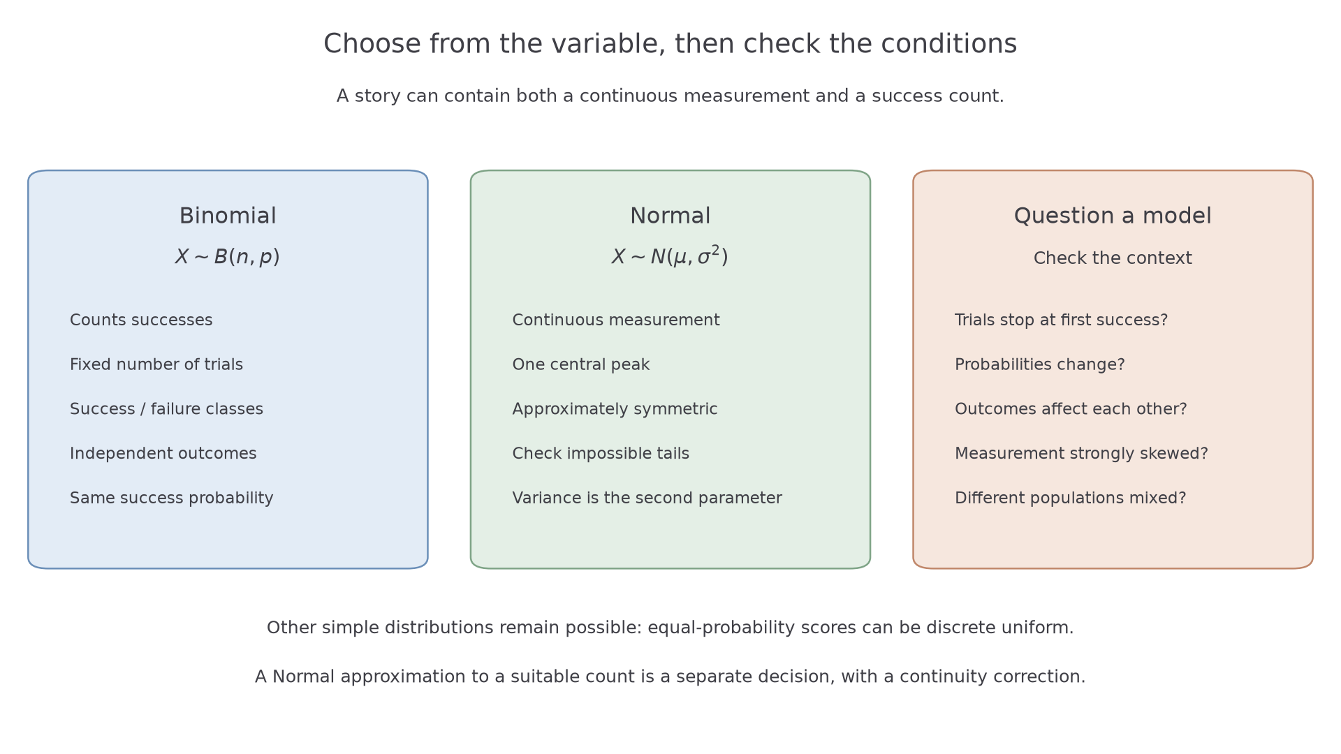
A model-choice answer includes both the distribution and its reason. “Neither Binomial nor Normal” can be sensible, but it does not mean that no probability distribution exists: a fair die score is a simple counterexample.

Key idea

Define the variable first, then test the proposed model's conditions in the actual situation.

Here the story stays fixed and the variable changes.

When a Binomial model is suitable

A packet either contains a prize or does not. Count prize packets in a fixed box, and the Binomial conditions become concrete statements about how the packets were filled.

A suitable Binomial model

$X\sim B(n,p)$ is suitable when $X$ counts successes in a fixed number $n$ of trials, each trial is classified as success or failure, trials are independent, and every trial has the same success probability $p$ .

An outcome can have many physical forms yet still be classified into two groups. A six-sided die gives “six” or “not six” when that is the chosen event. By contrast, the sum of the scores is not a success count.

Worked example 1: prize packets

Question. A box contains $40$ packets. Each packet independently contains a prize with probability $\frac17$ . Let $T$ count the prize packets. State a suitable distribution and justify it.

Plan. Match each Binomial condition to the packet situation.

\begin{aligned} n&=40 &&\text{fixed number of packets}\\ p&=\frac17 &&\text{same prize probability per packet}\\ T&\sim B\left(40,\frac17\right) &&\text{count independent prize outcomes} \end{aligned}

Why does “contains a prize” define a success? It is exactly the outcome $T$ counts; every other packet is a failure for this model.

Answer. $T\sim B(40,\frac17)$ : each of the $40$ fixed trials is prize/no prize, with independent outcomes and the same prize probability.

Check. $T$ takes integer values from $0$ to $40$ , matching possible box counts.

Change only the number of packets. The success event, probability and independence stay the same.

Worked example 2: a larger box

Question. A box now contains $50$ packets, filled independently with the same prize probability $\frac17$ . Let $U$ count prize packets. State a suitable distribution and the possible values of $U$ .

Plan. Replace the fixed trial count while retaining the success probability.

\begin{aligned} n&=50,\qquad p=\frac17 &&\text{change the trial count only}\\ U&\sim B\left(50,\frac17\right) &&\text{retain the same trial mechanism}\\ U&\in\{0,1,\ldots,50\} &&\text{count successes in fifty trials} \end{aligned}

Why is $p$ unchanged? It describes one packet, rather than the chance of a prize somewhere in the box.

Answer. $U\sim B(50,\frac17)$ , with possible counts $0$ through $50$ .

Check. The largest possible success count equals the number of trials; $U=51$ cannot occur.

A marketing problem works the same way: $120$ independent customer responses, each with order probability $0.18$ , give an order count modelled by $B(120,0.18)$ . Customers influencing one another would challenge that assumption.

Exam tip

If fixed trial count and success/failure are already given, an assumption question usually needs the remaining contextual condition: independent packet outcomes or constant prize probability.

Increase the box size again without changing the filling mechanism.

When a Normal model is suitable

For an individual measurement, look at shape before choosing the Normal notation. A histogram with one approximately symmetric bell-shaped mound is supporting evidence; a mean and standard deviation alone are not.

A suitable Normal model

A continuous measurement $X$ may be modelled by $N(\mu,\sigma^2)$ when its distribution is approximately symmetric and bell-shaped, and the model does not assign material probability to impossible values in its intended use.

Natural variation in lengths, masses or measurement errors can fit this pattern. Combining distinct groups can spoil it, so specify the population whose measurements you are modelling.

Worked example 3: an individual apple mass

Question. Apple mass $W$ , in grams, in one large crop has mean $164$ and standard deviation $18$ . A large random sample gives an approximately symmetric bell-shaped histogram. State a suitable model and justify it.

Plan. Check that mass is continuous and the observed shape fits, then square the standard deviation for the second parameter.

\begin{aligned} \mu&=164,\qquad \sigma=18 &&\text{identify the supplied summaries}\\ \sigma^2&=18^2=324 &&\text{write variance in the notation}\\ W&\sim N(164,324) &&\text{use the supporting histogram shape} \end{aligned}

Why is the histogram needed? Many skewed distributions can have these same summary values.

Answer. $W\sim N(164,18^2)$ , since mass is continuous and the sampled crop's histogram is approximately symmetric and bell-shaped.

Check. The mean is over nine standard deviations above zero, so impossible negative masses have negligible model probability.

Change only the standard deviation. The shape evidence and mean are unchanged.

Worked example 4: a less variable crop

Question. Another crop has the same mean $164\,\mathrm g$ and the same approximately symmetric bell-shaped distribution, but standard deviation $12\,\mathrm g$ . State a suitable model for mass $W$ and describe the change in its curve.

Plan. Keep the mean, replace the variance and compare spread at equal total area.

\begin{aligned} \mu&=164,\qquad \sigma=12 &&\text{change spread only}\\ W&\sim N(164,12^2)=N(164,144) &&\text{use the new variance} \end{aligned}

Why does the peak rise? Both curves enclose area $1$ ; concentrating the area into a narrower range makes the curve taller.

Answer. Use $N(164,144)$ . Its curve has the same centre, but is narrower and taller than the first crop's curve.

Check. $12<18$ , so the new model represents less variation; its second parameter $144$ is also smaller than $324$ .

For tomatoes with mean $82\,\mathrm g$ , standard deviation $9\,\mathrm g$ and a similar histogram, the corresponding notation is $N(82,9^2)$ . Changing the food does not alter the decision rule; changing the shape might.

Watch out

“Mass is continuous” is only part of the reason. A continuous waiting time can be strongly skewed, so continuity alone does not justify Normal symmetry.

Change only the standard deviation once more.

Recognising when the model is not appropriate

A convincing rejection names the failed condition. A fair spinner with scores $1$ to $8$ gives two useful counterexamples to an automatic Binomial choice.

Let $A$ be the number of spins until the first $7$ . The number of trials is not fixed in advance: it depends on the outcomes. Thus $A$ is not a Binomial success count. Let $B$ be the score on one spin. It takes the values $1,2,\ldots,8$ ; it is a discrete uniform score, rather than a count of successes.

Neither of these small-range or stopping-time variables is naturally described by a continuous Normal curve. Do not turn that into the rule “discrete means no Normal approximation”: large suitable Binomial counts are an important exception.

A failed model condition

A failed condition is a specific mismatch between the proposed model and the variable or trial mechanism, such as a changing success probability, dependent trials, an unfixed trial count, or an asymmetric measurement distribution.

Drawing without replacement from a small population changes probabilities. Counting emails received in a lunch break does not provide a fixed number of success/failure trials. A model for that count would need more information; there is no reason to assert that it is a nearly symmetric large count suitable for Normal approximation.

For Normal models, a long right tail conflicts with symmetry. Two peaks can indicate mixed populations. A nearby hard boundary matters if the proposed model places substantial probability beyond it; a distant boundary with negligible tail probability need not matter.

Key idea

Reject a model for its specific mismatch, and recognise when another simple distribution remains valid.

This example separates “fixed trials” from “constant probability”.

Continue this lesson.

You’re previewing NovaLearn without an account. Create a free account to read the rest.

Create free account

Last Accessed

Pure Mathematics (Papers 1 and 2)

Statistics (Paper 3, Section A)

Mechanics (Paper 3, Section B)

Statistics 4.3 - Choosing an appropriate probability distribution

Model choice starts with the random variable

When a Binomial model is suitable

When a Normal model is suitable

Recognising when the model is not appropriate

Continue this lesson.

Learn faster with Nova