Statistics 5.2 - Hypothesis test for a binomial proportion | Edexcel A-Level Mathematics

A high sample proportion can be evidence of a population change, but how high is high enough? You will carry out exact binomial tests, choose inclusive tails, find critical regions and explain their actual significance. You will also check whether the sampling and binomial assumptions support the conclusion.

From sample count to population proportion

A delivery company claims that $18\%$ of parcels arrive late. If $15$ out of $50$ arrive late, is that enough evidence of an increase? The observed $30\%$ is a starting point, not yet a verdict.

You already know

Under a binomial model there are a fixed number of independent trials, each with two outcomes and the same success probability. A hypothesis test calculates probabilities assuming $H_0$ , then judges the evidence in the direction of $H_1$ .

Call an arrival “success” when it is late. The word success is just a label for the outcome being counted.

Population proportion

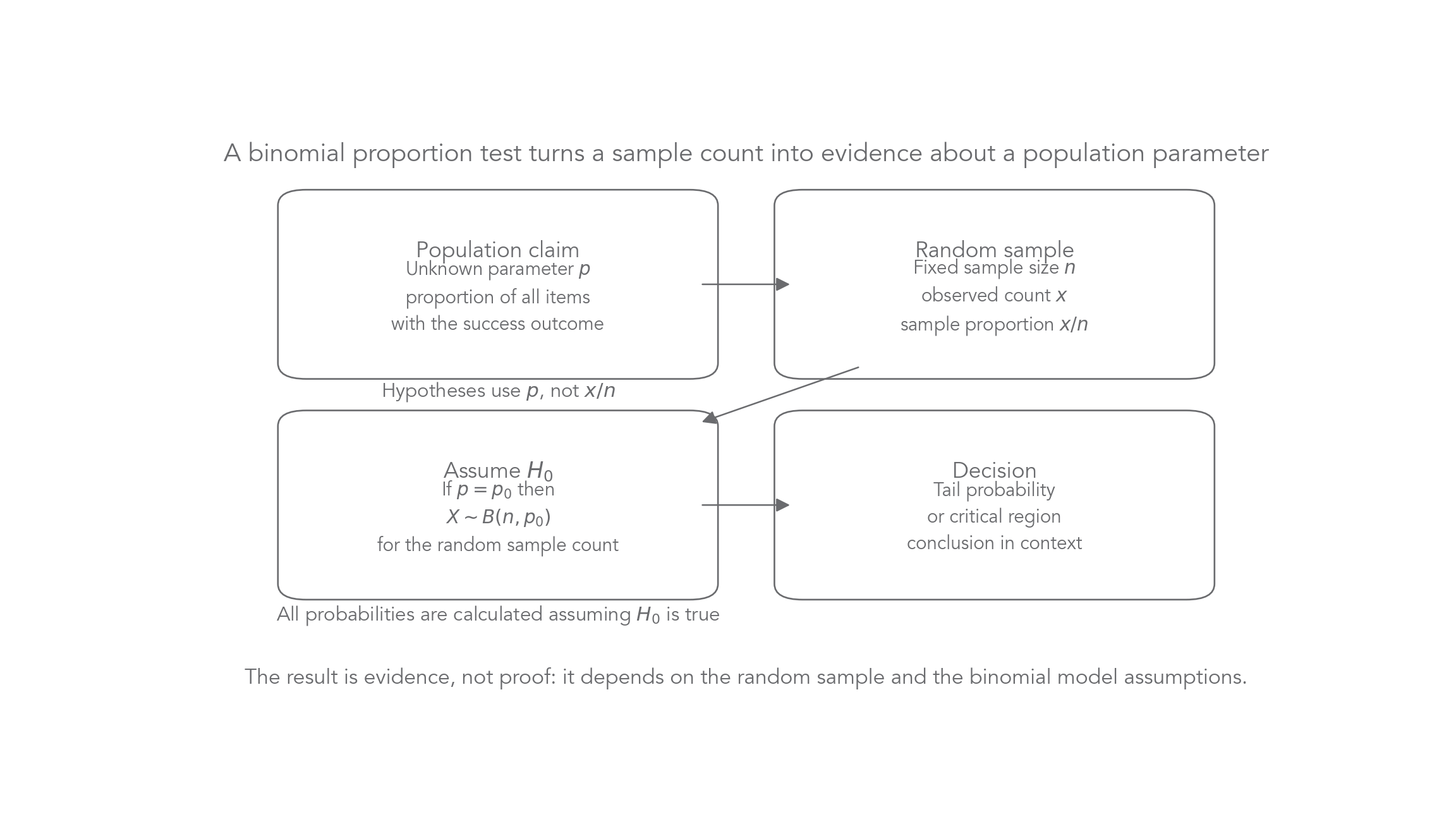
The population proportion $p$ describes the whole population, or the probability of success on one trial under the model. The observed sample proportion $x/n$ estimates $p$ ; it is not the parameter in the hypotheses.

If the null value is $p_0$ , the sample count has model $X\sim B(n,p_0)$ under $H_0$ . Define what $X$ counts, rather than listing calculator inputs without a distribution.

[DIAGRAM: asset_slug: p3_5_2_conduct_a_statistical_hypothesis_test_for_proportion_in_a_binomial_model__diagram_01; asset_name: Statistics 5.2 - Hypothesis test for a binomial proportion - diagram 01; caption: Sample evidence is judged under a population claim.; description: A flow diagram distinguishes the population parameter p, observed sample proportion x/n, null binomial distribution and contextual decision.]

Worked example 1: define the claim and evidence

Question. Set up an increased-lateness test for the delivery company and its random sample of $50$ parcels, containing $15$ late arrivals.

Plan. Define the population proportion, then use the claimed value in the count distribution.

\begin{aligned} p&=\text{proportion of all company parcels arriving late} &&\text{parameter}\\ H_0&:p=0.18\qquad H_1:p>0.18 &&\text{increase is the claim}\\ X&=\text{late parcels among the 50 sampled} &&\text{statistic}\\ X&\sim B(50,0.18)\text{ under }H_0 &&\text{claimed probability}\\ x/50&=15/50=0.30 &&\text{observed sample proportion} \end{aligned}

Why use $0.18$ in the model? The test asks whether $15$ would be unusually high if the old proportion still applied.

Answer. Test the unknown population $p$ , using observed count $15$ .

Check. The distribution's count runs from $0$ to $50$ ; both $15$ and $0.30$ have different roles.

Change only the sample size to $100$ , keeping $15$ late arrivals. This changes the statistic's distribution and the sample proportion, but not the population claim.

Worked example 2: a larger sample with the same count

Question. Set up the same increased-lateness test after $15$ late arrivals among $100$ sampled parcels.

Plan. Keep $p$ and the hypotheses, and replace the number of trials.

\begin{aligned} H_0&:p=0.18\qquad H_1:p>0.18 &&\text{unchanged claim}\\ X&\sim B(100,0.18)\text{ under }H_0 &&\text{new sample size}\\ x/100&=15/100=0.15 &&\text{new sample proportion} \end{aligned}

Why not change $H_1$ to a decrease? The investigator's original claim determines the alternative, not whichever direction this sample happens to take.

Answer. The observed proportion is now below the null value and does not point towards the suspected increase.

Check. The expected null count rises from $50(0.18)=9$ to $100(0.18)=18$ .

A representative random sample is needed to carry the evidence back to the intended population.

Watch out

Do not write $H_0:p=15/50$ after observing the sample. That would make the data define the claim they are meant to test.

Set up a lower-tail test in a new context.

Choosing the correct tail

If a new process is meant to reduce defects, a very small defective count supports its claim. A very large count does not support that claim, however unusual it is.

Wording	Alternative	Evidence to calculate
reduced, fewer, less	$p<p_0$	$P(X\le x)$
increased, more, greater	$p>p_0$	$P(X\ge x)$
changed, different	$p\ne p_0$	both tails, following the stated allocation

The observed value belongs in its own tail. For an upper tail, subtract the cumulative probability ending one count before it.

Inclusive upper binomial tail

For an integer observed count $x$ ,

P(X\ge x)=1-P(X\le x-1).

Not in the formula booklet: learn it.

This is the complement rule applied to whole-number counts. It avoids the most common calculator boundary slip.

Worked example 3: a reduced defect rate

Question. A factory's claimed defect rate is $4\%$ . A new process is intended to reduce it. There are $2$ defects in $120$ independently sampled items. State the hypotheses and the tail probability to use.

Plan. Translate “reduce” into a lower alternative and include the observed count.

\begin{aligned} H_0&:p=0.04\qquad H_1:p<0.04 &&\text{population defect probability}\\ X&\sim B(120,0.04) &&\text{null count distribution}\\ \text{tail probability}&=P(X\le2) &&\text{2 defects or fewer}\\ &=0.1371726\ldots &&\text{binomial cumulative calculation} \end{aligned}

Why not use $P(X=2)$ ? Counts $0$ and $1$ support a reduction even more strongly and must also be counted.

Answer. This is a one-tailed lower-tail test, using $P(X\le2)$ .

Check. The observed count $2$ is below the null expected count $120(0.04)=4.8$ .

Change only the suspected direction from reduction to increase. Even with the same observed count, the relevant probability changes.

Worked example 4: an increase uses the other tail

Question. Keep the same data, but investigate whether the defect probability has increased.

Plan. Change the alternative and take the inclusive upper tail.

\begin{aligned} H_0&:p=0.04\qquad H_1:p>0.04 &&\text{new direction}\\ P(X\ge2)&=1-P(X\le1) &&\text{include the observed 2}\\ &=0.9552597\ldots &&\text{not unusual in this direction} \end{aligned}

Why is the probability large? Two defects is not a high count compared with the expected $4.8$ .

Answer. Use the upper tail, and this sample does not supply evidence of an increase at $5\%$ .

Check. The tails $X\le2$ and $X\ge2$ overlap at $2$ , so their probabilities need not add to $1$ .

Choose the direction from the question before interpreting the data.

Watch out

$1-P(X\le x)$ means $P(X>x)$ , not $P(X\ge x)$ . An off-by-one error changes which sample outcomes count as evidence.

Now identify a claim with no preferred direction.

Using a tail probability as a p-value

A bakery's seeded-loaf share was $35\%$ . After a new display, $28$ of $60$ randomly sampled customers choose seeded loaves. The change looks promising; the null tail tells you how much evidence it provides.

For a one-tailed test, reject when the inclusive tail probability is at or below the chosen significance level. The significance level is selected in advance, not adjusted to make a preferred conclusion significant.

Worked example 5: a bakery's claim

Question. Test whether the population seeded-loaf proportion has increased, at the $5\%$ level. Treat customers' choices as independent with constant probability.

Plan. State population hypotheses and calculate the upper null tail.

\begin{aligned} H_0&:p=0.35\qquad H_1:p>0.35 &&\text{seeded-loaf population proportion}\\ X&\sim B(60,0.35) &&\text{count under }H_0\\ P(X\ge28)&=1-P(X\le27) &&\text{28 or more}\\ &=0.0411572\ldots<0.05 &&\text{significant} \end{aligned}

Why use the claimed $0.35$ ? You judge whether these purchases would be unusual if the display had not changed the population proportion.

Answer. Reject $H_0$ . There is sufficient evidence at $5\%$ that the population proportion choosing seeded loaves has increased.

Check. The sample count $28$ exceeds the expected $60(0.35)=21$ , agreeing with the upper-tail direction.

Change only the observed count to $29$ . Leave the significance level alone.

Worked example 6: stronger evidence from one more purchase

Question. Repeat the same test with $29$ seeded-loaf purchases among $60$ customers.

Plan. Move the inclusive tail boundary by one count.

\begin{aligned} P(X\ge29)&=1-P(X\le28) &&\text{new observed boundary}\\ &=0.0228343\ldots<0.05 &&\text{same decision at 5 per cent} \end{aligned}

Why is this stronger evidence? A still larger count is less likely under the unchanged null model.

Answer. Reject $H_0$ ; there is sufficient evidence of an increased population seeded-loaf proportion.

Check. Both tests reject at $5\%$ , but only the second rejects at $2.5\%$ : $0.0228343<0.025<0.0411572$ .

The evidence concerns a proportion, not an assertion that a particular future customer will buy the loaf.

Exam tip

Write the probability statement beside the calculator result, then compare it with the correct threshold. Finish with “sufficient” or “insufficient evidence” and the population claim in context.

Carry out a test using a supplied probability.

Continue this lesson.

You’re previewing NovaLearn without an account. Create a free account to read the rest.

Create free account

Last Accessed

Pure Mathematics (Papers 1 and 2)

Statistics (Paper 3, Section A)

Mechanics (Paper 3, Section B)

Statistics 5.2 - Hypothesis test for a binomial proportion

From sample count to population proportion

Choosing the correct tail

Using a tail probability as a p-value

Continue this lesson.

Learn faster with Nova