Pure 2.11 - Functions in modelling | Edexcel A-Level Mathematics

A function model links a real input to a predicted output. Learn to interpret its constants, choose a suitable family, fit it to data and decide where its predictions can be trusted. A useful refinement changes a particular weakness in the model.

What a function model says

Can a cooling drink end up colder than the room in a model that is supposed to describe ordinary cooling? A straight-line prediction can say yes. The algebra may be correct while the model needs changing; by the end, you will be able to explain and repair that mismatch.

First consider $T(t)=18+62e^{-0.08t}$ , where $T$ is temperature in degrees Celsius and $t$ is minutes since pouring. At the start it predicts $18+62=80$ , while much later it approaches $18$ .

You already know

Substitution evaluates a function, $e^0=1$ , and a negative exponential $e^{-kt}$ , $k>0$ , approaches zero as $t$ increases. A horizontal translation or vertical shift changes a graph's position.

The equation alone is incomplete: its variables, units, allowed inputs and assumptions tell you what it describes.

Function model

A function model is a simplified rule predicting one quantity from another. Variables change within the model; parameters are constants controlling its behaviour. The contextual domain contains the input values for which the situation and assumptions make sense.

The cooling rule is mathematically defined for all real $t$ , but negative time is outside “minutes since pouring”. Even $t\ge0$ need not guarantee reliability: the room temperature might change later.

Worked example 1: interpret initial and limiting values

Question. For $T(t)=18+62e^{-0.08t}$ , $0\le t\le60$ , find the initial temperature and interpret $18$ .

Plan. Substitute zero, then consider what happens as the exponential becomes small.

\begin{aligned} T(0)&=18+62e^0 &&\text{initial input}\\ &=80 &&\text{use }e^0=1\\ e^{-0.08t}&\to0\text{ as }t\to\infty &&\text{exponential decay}\\ T(t)&\to18 &&\text{limiting value of the rule} \end{aligned}

Why distinguish the two constants? The added $18$ is the limiting temperature; the $62$ is the initial excess above it.

Answer. The initial temperature is $80$ degrees Celsius; $18$ represents room temperature. The limiting behaviour describes the mathematical rule, beyond its stated $60$ -minute use interval.

Check. The predicted starting temperature exceeds the room temperature by $62$ degrees Celsius.

Change only the initial excess from $62$ to $52$ . The surrounding temperature and decay parameter stay fixed.

Worked example 2: a different initial excess

Question. Interpret the initial and limiting temperatures in $S(t)=18+52e^{-0.08t}$ , $0\le t\le60$ .

Plan. Apply the same zero-input and long-term checks.

\begin{aligned} S(0)&=18+52(1)=70 &&\text{initial temperature}\\ S(t)-18&=52e^{-0.08t}>0 &&\text{positive for finite }t\\ S(t)&\to18 &&\text{exponential term tends to zero} \end{aligned}

Why is the curve above room temperature? The excess stays positive even as it becomes smaller.

Answer. Initially $70$ degrees Celsius, tending towards $18$ degrees Celsius under unchanged conditions.

Check. At $t=0$ , the excess $70-18=52$ matches the coefficient.

A pleasant mathematical surprise is that these two drinks have the same proportional cooling of their excess: after $10$ minutes each excess is multiplied by $e^{-0.8}\approx0.449$ . The total temperatures are not multiplied by that factor, because the room-temperature offset stays.

Watch out

The wrong statement “the initial temperature is $18$ ” ignores the exponential term at zero. Always calculate $T(0)$ before interpreting a parameter.

Change the initial excess once more for this short interpretation.

Choosing a function family

Look for the pattern before selecting a rule. Repetition suggests a trigonometric model; constant percentage change suggests an exponential; a constant product suggests inverse proportion.

Pattern	Family and form	Meaning to check
tide or annual daylight cycle	$y=M+A\cos(\frac{2\pi(t-h)}P)$	midline $M$ , amplitude $
growth or decay by a fixed factor in equal intervals	$y=ab^t$ , $a>0,b>0$ , or $ae^{kt}$	initial value and growth/decay rate
inverse proportion	$y=k/x$ , $x>0$ in many applications	constant product $xy=k$

For the cosine form shown, take $A>0$ when $h$ is the time of a maximum. All angles here are in radians. The midline, amplitude and period formulas used for these models are not in the formula booklet: learn them.

[DIAGRAM: asset_name: Three function model families; asset_slug: p1_2_11_use_functions_in_modelling_and_appreciate_their_limitations_and_refinements__diagram_01; caption: Repetition, constant percentage decay and inverse proportion; description: Three graphs show the constructed tide D=7+3cos(pi t/6), exponential C=20exp(-0.3t) and gas model P=240/V, with their important features labelled.]

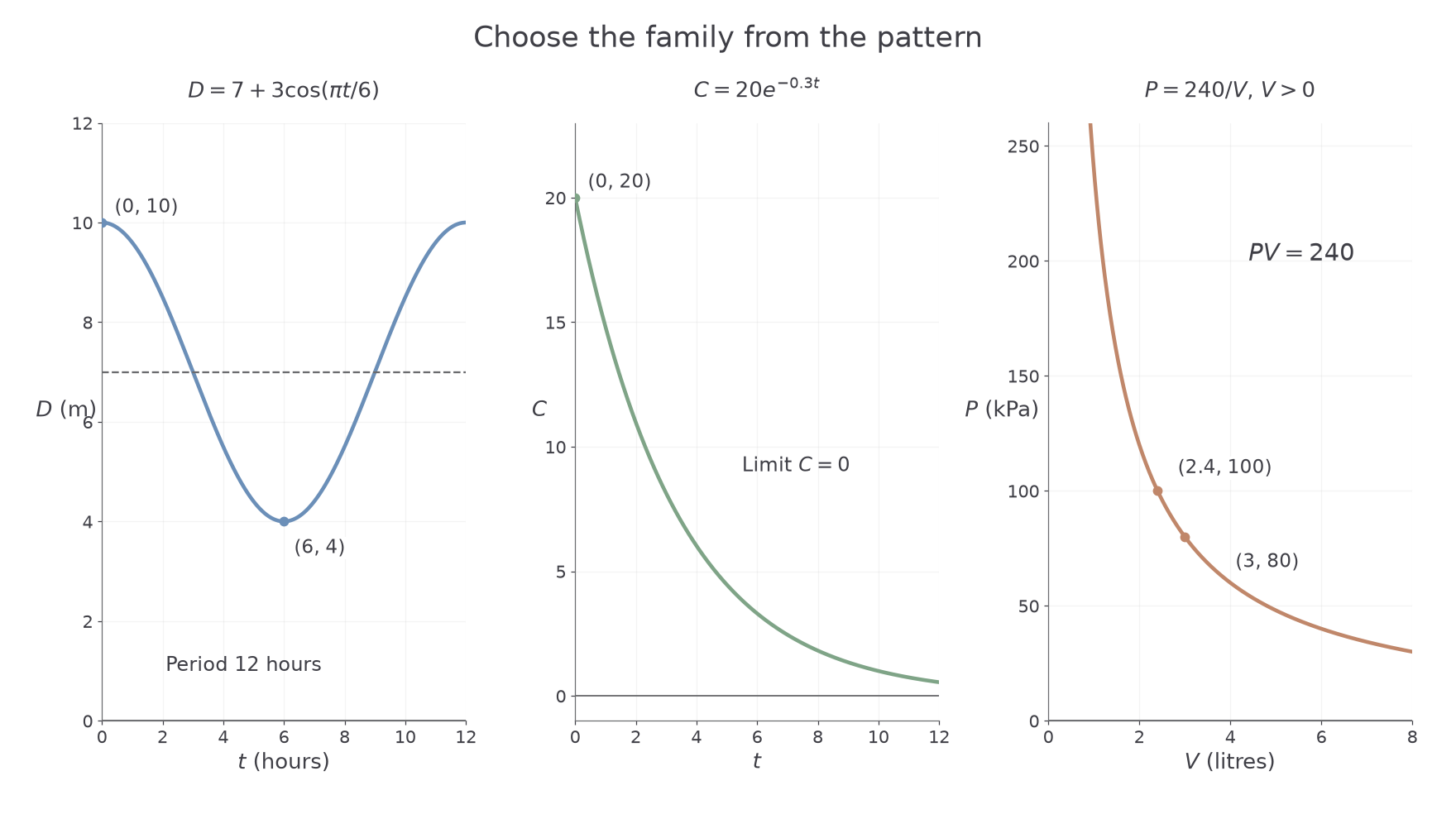
These are constructed examples, rather than measurements from a named harbour or experiment. For a fixed amount of gas at constant temperature, the simple inverse model $P=\frac{240}V$ predicts $80\,\mathrm{kPa}$ at $V=3$ litres and $100\,\mathrm{kPa}$ at $V=2.4$ litres. Both products $PV$ equal $240$ ; the physical assumptions are essential.

Worked example 3: fit a repeating cycle

Question. A harbour depth is modelled with maximum $10\,\mathrm m$ at midnight, minimum $4\,\mathrm m$ six hours later and period $12$ hours. Find a cosine model for depth $D$ metres, $t$ hours after midnight, $0\le t\le12$ .

Plan. Average the extremes for the midline, halve their difference for the amplitude and use cosine at its maximum.

\begin{aligned} M&=(10+4)/2=7 &&\text{midline}\\ A&=(10-4)/2=3 &&\text{amplitude}\\ \omega&=2\pi/12=\pi/6 &&\text{one cycle per }12\text{ hours} \end{aligned}

Why use cosine without a shift? It equals $1$ at the starting maximum.

Answer. $D(t)=7+3\cos(\frac{\pi t}6)$ , $0\le t\le12$ .

Check. $D(0)=10$ , $D(6)=4$ , $D(12)=10$ .

Change only the time of high tide, delaying the same cycle by two hours. The heights and period remain fixed.

Worked example 4: move the cycle in time

Question. With the same extremes and period, high tide occurs at $t=2$ , low tide at $t=8$ . Find a model on $2\le t\le14$ .

Plan. Keep the midline and amplitude, replacing $t$ by $t-2$ .

\begin{aligned} M&=7,\quad A=3,\quad\omega=\pi/6 &&\text{unchanged shape}\\ D(t)&=7+3\cos\left(\frac{\pi(t-2)}6\right) &&\text{delay by two hours} \end{aligned}

Why subtract inside? At $t=2$ , the cosine must receive zero to put the peak there.

Answer. $D(t)=7+3\cos(\frac{\pi(t-2)}6)$ , $2\le t\le14$ .

Check. $D(2)=10$ , $D(8)=4$ , $D(14)=10$ .

Daylight can be modelled similarly: extremes $16$ and $8$ hours, with period $12$ months and a maximum at $t=0$ , give $12+4\cos(\frac{\pi t}6)$ . A fixed sinusoid assumes identical cycles and ignores irregular weather effects on tides or gradual changes in the underlying pattern.

Watch out

A constant percentage increase is not a constant amount increase. For instance, multiplying by $1.1$ each interval is exponential; adding $0.1$ each interval is linear.

Change only the high-tide timing again.

Fitting constants and using a model

A proposed form becomes a usable model when observations determine its constants. Keep exact values during fitting, then round the prediction. For $V=pe^{kt}$ , the parameter $p$ is the initial value; $k>0$ gives growth and $k<0$ gives decay.

You already know

Natural logarithms reverse exponentials: $e^u=v$ gives $u=\ln v$ , for $v>0$ . Divide by a multiplier before taking logarithms; $15000=24000e^{4k}$ first becomes $e^{4k}=15000/24000$ .

This inverse operation turns an unknown exponent into an ordinary linear equation.

Fit an exponential from two observations

If $V(0)=V_0>0$ and $V(T)=V_T>0$ , $T>0$ , in the model $V=pe^{kt}$ , then

p=V_0,\qquad k=\frac1T\ln\left(\frac{V_T}{V_0}\right).

This follows by dividing $V_T=V_0e^{kT}$ by $V_0$ and taking logarithms.

Not in the formula booklet: learn it.

You can equivalently write $V=V_0(\frac{V_T}{V_0})^{t/T}$ ; it makes the observed time interval particularly clear.

Worked example 5: fit depreciation

Question. A machine's value $V$ pounds, $t$ years after purchase, follows $V=pe^{kt}$ . It costs $\pounds24{,}000$ and is worth $\pounds15{,}000$ after four years. Find the model and predict its value after six years.

Plan. Use the initial value for $p$ , then solve the four-year equation for $k$ .

\begin{aligned} p&=24000 &&\text{set }t=0\\ 15000&=24000e^{4k} &&\text{use the second observation}\\ k&=\tfrac14\ln(5/8) &&\text{divide and take logs}\\ V(6)&=24000(5/8)^{6/4} &&\text{predict with exact constants}\\ &=11858.541\ldots &&\text{evaluate} \end{aligned}

Why avoid rounding $k$ first? The rounded rate would be exponentiated, reducing the accuracy of the final value.

Answer. $V=24000(\frac58)^{t/4}$ , predicting about $\pounds11{,}900$ after six years, to $3$ significant figures.

Check. $V(4)=24000\cdot\frac58=15000$ ; the six-year value is smaller, consistent with decay.

Change only the observed four-year value, from $\pounds15{,}000$ to $\pounds12{,}000$ . The model now loses half its value in each four-year interval.

Worked example 6: a changed decay rate

Question. Fit the same model with initial value $\pounds24{,}000$ and four-year value $\pounds12{,}000$ , then predict the six-year value.

Plan. Replace the observed ratio, retaining the same fitting method.

\begin{aligned} p&=24000 &&\text{initial observation}\\ 12000&=24000e^{4k} &&\text{new four-year observation}\\ k&=\tfrac14\ln(1/2) &&\text{solve for the rate}\\ V(6)&=24000(1/2)^{3/2}=8485.281\ldots &&\text{predict at six years} \end{aligned}

Why is the new prediction lower? The observed retention factor $\frac12$ is smaller than $\frac58$ .

Answer. $V=24000(\frac12)^{t/4}$ , predicting $\pounds8{,}490$ to $3$ significant figures.

Check. The model gives $\pounds12{,}000$ at four years and $\pounds6{,}000$ at eight years, bracketing the six-year value.

The same fitting works for mass: an initial $80\,\mathrm{mg}$ falling to $50\,\mathrm{mg}$ in three hours gives $M=80(\frac58)^{t/3}$ , predicting $36.6\,\mathrm{mg}$ after five hours. Context changes the interpretation, not the algebra.

Exam tip

Use the stated model and give the prediction in context. A modelled resale value is an estimate, even when the calculation is exact.

Change the four-year observation once more for a matched fitting task.

Limitations and validity

A model can fit its observations and still fail later. Check the contextual domain, physically possible outputs and assumptions before trusting a prediction. For a battery model $B=100e^{-0.12t}$ , the initial output is $100\%$ , but extending to negative time predicts more than a full charge and lies outside “hours after charging”.

Interpolation and extrapolation

Interpolation predicts between observed input values. Extrapolation predicts outside their range. For example, a six-year prediction fitted from ages zero and four is extrapolation, even if it is mathematically defined.

Extrapolation is often less reliable because the assumptions may stop holding. A possible output is only a basic check, not proof that the model is accurate.

Worked example 7: find a physical contradiction

Question. Algae area $A$ , in square metres, follows $A=3e^{0.4t}$ , where $t$ is days. The lake surface is $200$ square metres. Predict the area at $t=12$ and assess the model there.

Plan. Calculate the prediction and compare it with the available surface.

\begin{aligned} A(12)&=3e^{4.8} &&\text{substitute the time}\\ &=364.531\ldots &&\text{evaluate}\\ 364.531\ldots&>200 &&\text{compare with the capacity} \end{aligned}

Why use the lake area? It supplies a real upper bound that the exponential model lacks.

Answer. The model predicts about $365$ square metres, which is impossible on a $200$ -square-metre surface, so it is unsuitable at this time.

Check. The prediction is more than the entire lake, not merely a small rounding excess.

Change only the prediction time to ten days. A smaller prediction removes that particular contradiction, without establishing reliability.

Worked example 8: distinguish possible from validated

Question. Use the same algae model at $t=10$ . Does the lake-area check establish that the model is accurate?

Plan. Evaluate and compare, then state what this check can actually show.

\begin{aligned} A(10)&=3e^4 &&\text{substitute}\\ &=163.794\ldots &&\text{evaluate}\\ 163.794\ldots&<200 &&\text{physically possible area} \end{aligned}

Why avoid concluding “accurate”? Passing one bound says nothing about whether the growth rate matches observations.

Answer. About $164$ square metres is possible, but accuracy still requires suitable observations and reasonable assumptions.

Check. $0<A(10)<200$ ; this is the check passed, rather than a validation of the entire model.

Likewise, $P=\frac{240}V$ needs $V>0$ , constant temperature and a fixed quantity of gas. Heating the gas changes the pressure relationship; very small volumes may expose the limits of the idealised inverse-proportion rule.

Key idea

Name the assumption or bound that fails, then connect it to the prediction. “The model is unrealistic” on its own does not explain anything.

Keep the same bound and change the prediction time once more.

Refining a model

A refinement changes a specific weakness. You might restrict the time interval, fit new parameters from more observations, add a limiting value, use different rules over different intervals or include an ignored variable. Choose the change that addresses the evidence.

Consider a drink initially at $90$ degrees Celsius in a room at $20$ degrees Celsius. A line can describe the first few minutes, but its constant decrease eventually carries it through room temperature. A shifted exponential can build in the limiting temperature.

Worked example 9: add a sensible limiting value

Question. Compare $L(t)=90-2.6t$ and $E(t)=20+70e^{-0.06t}$ for ordinary cooling, with $t$ in minutes. Calculate both at $t=30$ and explain the better long-term model.

Plan. Compare predictions with room temperature and inspect their limiting behaviour.

\begin{aligned} L(30)&=90-2.6(30)=12 &&\text{linear prediction}\\ E(30)&=20+70e^{-1.8}=31.570\ldots &&\text{exponential prediction}\\ E(t)&\to20 &&\text{excess tends to zero} \end{aligned}

Why add $20$ ? A model $90e^{-0.06t}$ would tend to zero rather than to the room temperature.

Answer. $L$ predicts $12$ degrees Celsius, below the room temperature; $E$ predicts $31.6$ degrees Celsius and tends towards $20$ . Under fixed room conditions, $E$ has the more suitable long-term behaviour.

Check. $E(0)=20+70=90$ ; the initial temperature is preserved.

Change only the room temperature to $25$ degrees Celsius, keeping the initial temperature and assumed decay parameter. This changes the limiting value and therefore the initial excess.

Worked example 10: refine the surrounding conditions

Question. Construct the corresponding cooling model for a drink initially at $90$ degrees Celsius in a room at $25$ degrees Celsius, keeping decay parameter $0.06$ . Predict its temperature after $30$ minutes.

Plan. Use $25$ as the limit and choose the excess to preserve the initial value.

\begin{aligned} 90-25&=65 &&\text{initial excess}\\ R(t)&=25+65e^{-0.06t} &&\text{refined model}\\ R(30)&=25+65e^{-1.8}=35.744\ldots &&\text{predict} \end{aligned}

Why change the coefficient too? Keeping $70$ would give an incorrect initial temperature of $95$ .

Answer. $R(t)=25+65e^{-0.06t}$ , predicting $35.7$ degrees Celsius after $30$ minutes.

Check. $R(0)=90$ , and $R(t)>25$ for every finite $t\ge0$ .

Holding the decay parameter fixed was an explicit modelling assumption, not a claim that changing room conditions never affects it. New temperature readings could estimate it again. For a daily cycle between $3$ and $9$ , the midline is $6$ , amplitude $3$ ; if the daily maximum changes with season, fitting separate seasonal models or a varying amplitude would address that weakness.

The opening question is now resolved. The drink can fall below room temperature in the linear equation because the equation assumes a constant cooling amount forever. A limiting-value refinement removes that contradiction under the stated physical assumptions.

Problem-solving

Connect each refinement to its purpose: a new limit fixes long-term behaviour; new observations improve fitted constants; a restricted domain avoids an unsupported prediction.

Change the surrounding temperature once more while preserving the initial condition.

Quick Recap

Define variables, units, parameters and the contextual domain before using a model.
Match repeated cycles, percentage change and constant products to suitable function families.
Fit constants from observations and keep exact values until the final prediction.
Check domain, physical bounds and assumptions; a possible output is not proof of accuracy.
Refine the specific feature that causes a failure.

The opening drink falls below room temperature only because the linear rule keeps subtracting a fixed amount. A shifted exponential preserves the initial temperature and approaches the room temperature instead.

Last Accessed

Pure Mathematics (Papers 1 and 2)

Statistics (Paper 3, Section A)

Mechanics (Paper 3, Section B)

Pure 2.11 - Functions in modelling