Statistics 5.1 - Language of statistical hypothesis testing | Edexcel A-Level Mathematics

How unusual must a sample be before you question a population claim? You will learn to set up hypotheses, recognise extreme results and make careful decisions using critical regions or p-values. The same language will then let you test a claim about linear correlation.

Hypotheses and test statistics

If a company says that $30\%$ of orders use a discount code, would $9$ code-users in $15$ orders make you doubt it? The sample proportion is $9/15=0.6$ , twice the claimed proportion. Sampling varies, though: the size of the disagreement alone does not settle the question.

You already know

A binomial random variable counts successes in a fixed number of independent trials with constant success probability. Under $X\sim B(n,p)$ , its expected value is $np$ .

Start by separating the claim from the evidence. A population parameter describes the population; a statistic is calculated from the sample.

Null and alternative hypotheses

The null hypothesis $H_0$ supplies the population model being tested. The alternative hypothesis $H_1$ describes the departure for which you seek evidence. For a proportion, write $H_0:p=p_0$ and choose $H_1:p>p_0$ , $p<p_0$ or $p\ne p_0$ from the question's claim.

The test statistic is the random quantity used to judge the evidence. Here it is the count $X$ ; the particular count you observe is $x$ . Equality in $H_0$ gives one definite model from which probabilities can be calculated.

Worked example 1: an increase in code use

Question. In the discount-code example, a manager suspects an increase. Define the parameter and statistic, state the hypotheses and give the null distribution.

Plan. Describe the whole population using $p$ , then model the sample count under the claimed proportion.

\begin{aligned} p&=\text{proportion of all orders using a code} &&\text{population parameter}\\ H_0&:p=0.30 &&\text{claimed model}\\ H_1&:p>0.30 &&\text{suspected increase}\\ X&=\text{code-users in 15 sampled orders} &&\text{test statistic}\\ X&\sim B(15,0.30)\text{ under }H_0 &&\text{fixed null probability} \end{aligned}

Why use $0.30$ , rather than $9/15$ , in the model? You are asking how surprising the sample is if the original claim holds.

Answer. The hypotheses concern $p$ ; the observed statistic is $x=9$ .

Check. The sample proportion $0.6$ is evidence about $p$ , not a value to substitute for $p_0$ .

Change only the manager's suspicion. The same data can be judged against a different question, but that question must be chosen before inspecting the result.

Worked example 2: a difference in either direction

Question. Keep the same company, claim and sample. The manager now wants to investigate whether code use has changed in either direction. Set up the test.

Plan. Keep the null model and change the alternative to match “changed”.

\begin{aligned} H_0&:p=0.30 &&\text{same population claim}\\ H_1&:p\ne0.30 &&\text{either direction matters}\\ X&\sim B(15,0.30)\text{ under }H_0 &&\text{same statistic and model} \end{aligned}

Why does the model stay the same? The alternative selects the evidence to look for; it does not replace the null probability.

Answer. This is a two-tailed test, still based on the observed count $9$ .

Check. Both unusually small and unusually large counts could now challenge $H_0$ .

Keep the population and sample symbols distinct when you set up the next test.

Watch out

$H_0:X=9$ is not a population hypothesis. The count $9$ has already been observed; the unknown quantity is the population proportion $p$ .

Try the same setup for a different claimed proportion.

Tails and critical regions

For $X\sim B(20,0.5)$ , you expect about $10$ successes. Counts near $0$ or $20$ look unusual; which of them matters depends on the alternative.

Alternative	Test	Evidence against the null
$p<p_0$	one-tailed	unusually small counts
$p>p_0$	one-tailed	unusually large counts
$p\ne p_0$	two-tailed	unusually small or large counts

The mean locates the centre; it is not a rejection boundary.

Expected binomial count

E(X)=np\qquad\text{for }X\sim B(n,p).

In the formula booklet.

Choose a significance level before collecting the evidence. It controls how readily you reject a true null model.

Significance level and critical region

The critical region is the set of statistic values leading to rejection of $H_0$ . Its boundary values are critical values. The significance level is the chosen probability limit for wrongly rejecting $H_0$ when it is true; a discrete test's actual rejection probability may be lower. Values outside the critical region form the acceptance region, meaning “do not reject”.

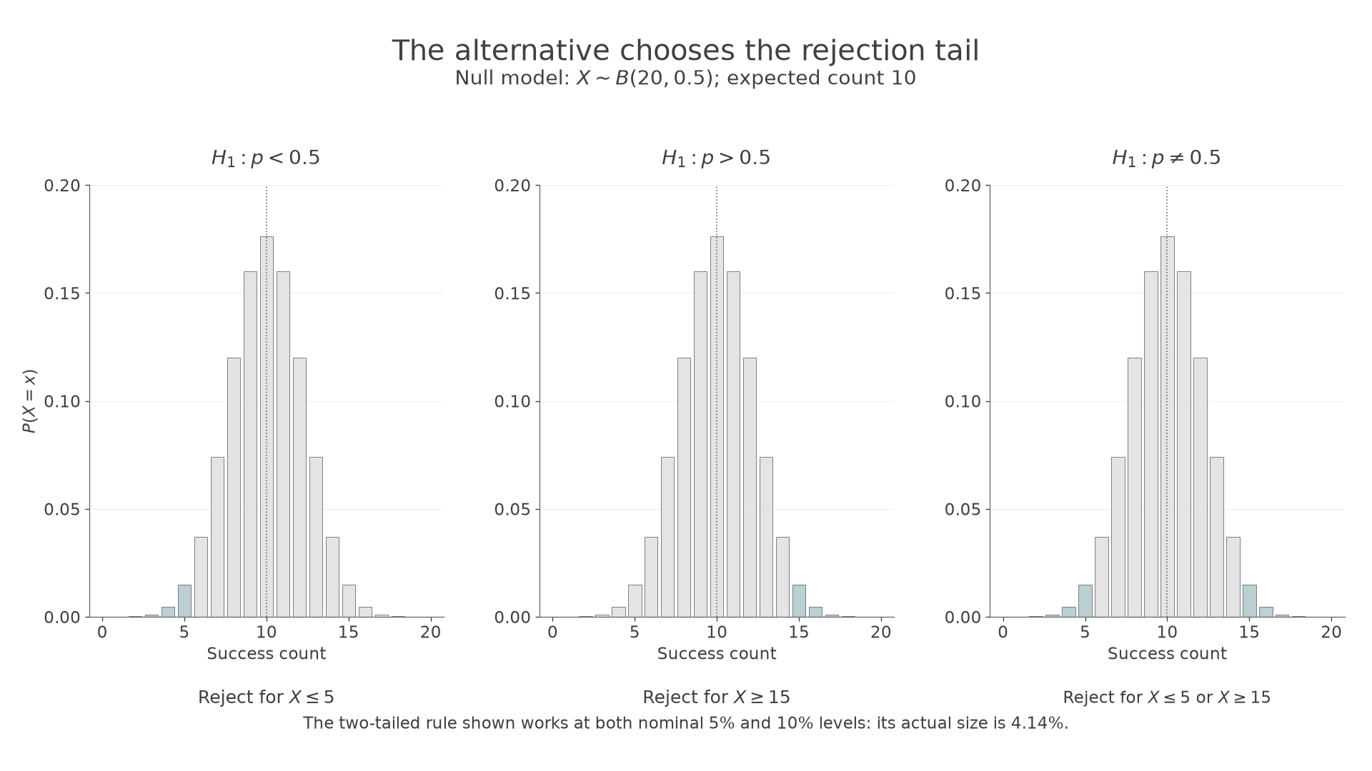
Here whole bars belong either inside or outside the rejection region. You cannot shade a fraction of one observed count.

[DIAGRAM: asset_slug: p3_5_1_understand_and_apply_the_language_of_statistical_hypothesis_testing__diagram_01; asset_name: Statistics 5.1 - Language of statistical hypothesis testing - diagram 01; caption: The alternative decides which counts are extreme.; description: Three binomial bar charts for B(20,0.5), showing lower, upper and two-tailed rejection regions with exact integer boundaries.]

Worked example 3: a two-tailed decision rule

Question. Find a critical region for a $10\%$ two-tailed test with null distribution $B(20,0.5)$ , putting at most $5\%$ in each tail. Give its actual significance level.

Plan. Find the largest lower-tail region within $0.05$ , then use symmetry.

\begin{aligned} E(X)&=20(0.5)=10 &&\text{locate the centre}\\ P(X\le5)&=0.0206947\ldots &&\text{within the tail allowance}\\ P(X\le6)&=0.0576591\ldots>0.05 &&\text{next bar is too much}\\ P(X\ge15)&=0.0206947\ldots &&\text{symmetry about 10} \end{aligned}

Why stop at $5$ ? Including $6$ would exceed the chosen probability limit for that tail.

Answer. Reject for $X\le5$ or $X\ge15$ . The critical values are $5$ and $15$ ; the acceptance region is $6\le X\le14$ . The actual significance is $2(0.0206947\ldots)=0.0413895\ldots$ , about $4.14\%$ .

Check. The actual probability is below the nominal $10\%$ .

Change only the nominal level to $5\%$ . Surprisingly, the decision rule need not change at all.

Worked example 4: the same bars at a different level

Question. Repeat the test with a nominal $5\%$ significance level and at most $2.5\%$ in each tail.

Plan. Compare the same adjacent tail probabilities with the new allowance.

\begin{aligned} P(X\le5)&=0.0206947\ldots<0.025 &&\text{still allowed}\\ P(X\le6)&=0.0576591\ldots>0.025 &&\text{still too large} \end{aligned}

Why are the boundaries unchanged? There is no whole-number boundary between $5$ and $6$ .

Answer. The critical region remains $X\le5$ or $X\ge15$ , with actual significance about $4.14\%$ .

Check. This actual probability fits both nominal levels. Discreteness explains the apparent surprise.

An acceptance region is a decision set, not a proof that the population claim is correct.

Watch out

Write a critical region as values, such as $X\le5$ , not as a probability such as $P(X\le5)$ . The probability measures how often the region is reached; it is not the region itself.

Use symmetry again, this time with a smaller sample.

P-values and conclusions

Suppose a task has claimed success probability $0.4$ , but you succeed $7$ times in $10$ attempts. A p-value measures how surprising this count or a more extreme count would be under the claim.

p-value

A p-value is the probability, calculated assuming $H_0$ , of the observed statistic or something at least as extreme in the direction of $H_1$ . It is not the probability that $H_0$ is true.

For an upper-tail binomial test, include the observed count: $P(X\ge x)=1-P(X\le x-1)$ . For a lower-tail test, use $P(X\le x)$ . These are tail probabilities, not the probability of just one count.

Worked example 5: just outside significance

Question. Test $H_0:p=0.4$ against $H_1:p>0.4$ at the $5\%$ level after $7$ successes in $10$ independent attempts.

Plan. Calculate the upper tail under $H_0$ , then compare it with $0.05$ .

\begin{aligned} X&\sim B(10,0.4) &&\text{null model}\\ P(X\ge7)&=1-P(X\le6) &&\text{include 7 and larger counts}\\ &=0.0547619\ldots>0.05 &&\text{not sufficiently unusual} \end{aligned}

Why use the upper tail? Only higher success probabilities support the stated alternative.

Answer. Do not reject $H_0$ . There is insufficient evidence at the $5\%$ level that the task's success probability exceeds $0.4$ .

Check. A sample proportion $0.7$ is above $0.4$ , but this small sample has not crossed the chosen evidence threshold.

Change only the observed count to $8$ . That one extra success removes a whole bar from the upper-tail probability.

Continue this lesson.

You’re previewing NovaLearn without an account. Create a free account to read the rest.

Create free account

Last Accessed

Pure Mathematics (Papers 1 and 2)

Statistics (Paper 3, Section A)

Mechanics (Paper 3, Section B)

Statistics 5.1 - Language of statistical hypothesis testing

Hypotheses and test statistics

Tails and critical regions

P-values and conclusions

Continue this lesson.

Learn faster with Nova