Pure 2.7 - Graphs of functions and the modulus graph | Edexcel A-Level Mathematics

A useful sketch records what a function does without calculating every point. Learn to build polynomial, modulus, reciprocal and proportion graphs from their key features, then read equations and inequalities as intersections and relative heights.

Sketching simple polynomial graphs

Can a quartic have two different roots and never cross the horizontal axis? Try $y=x^2(2x-1)^2$ : its value is a product of squares, so it cannot be negative. Its roots must be touches, rather than crossings. We will use a few features to explain the whole shape.

You already know

A product is zero when at least one factor is zero. Substituting $x=0$ gives the vertical-axis intercept; expanding the highest-power factors gives the leading term.

At an odd-multiplicity root, the sign changes as you pass through it. At an even-multiplicity root, it does not. A simple root crosses; a double root touches and turns. A triple root crosses with a flattened shape.

Root and multiplicity

A root $r$ satisfies $f(r)=0$ . Its multiplicity is the power of $(x-r)$ in the fully factorised polynomial. For example, $(x+2)(x-1)^2$ has a simple root $-2$ and a double root $1$ .

The leading term controls the distant ends. A positive cubic falls to the left and rises to the right; a positive quartic rises at both ends. A negative leading coefficient reverses those directions. These graph rules are not in the formula booklet: learn them.

[DIAGRAM: asset_name: Cubic crossings and quartic touches; asset_slug: p1_2_7_understand_and_use_graphs_of_functions_including_functions_defined_by_simple_polynomials_and_the_modulus_graph__diagram_01; caption: Multiplicity controls crossing or touching; description: The cubic (x+2)(x-1)(x-3) crosses at -2, 1 and 3. The quartic x squared times (2x-1) squared touches at 0 and one half and stays non-negative.]

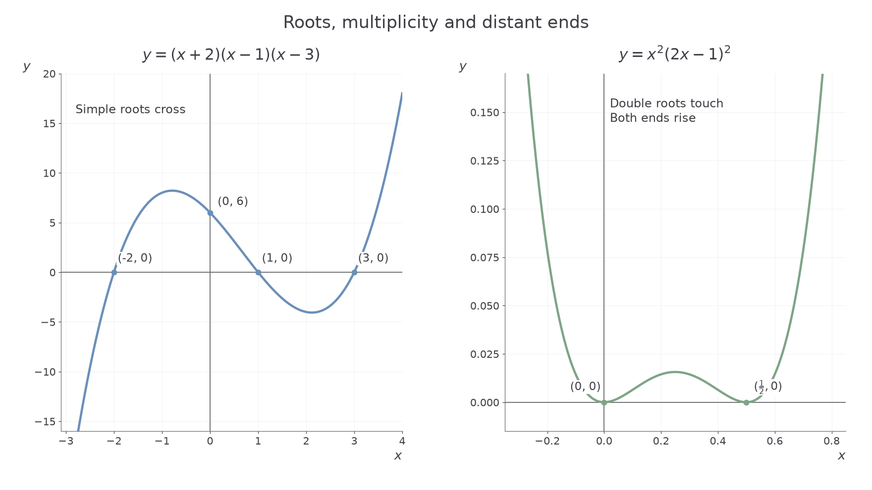
A sketch needs roots, the vertical intercept and consistent ends; exact turning points are unnecessary unless requested.

Worked example 1: read a factorised cubic

Question. Describe the key features of $y=(x+2)(x-1)(x-3)$ .

Plan. Read roots from factors, evaluate at zero and use the leading term for the ends.

\begin{aligned} y=0&\implies x=-2,1,3 &&\text{set each factor to zero}\\ y(0)&=2(-1)(-3)=6 &&\text{vertical intercept}\\ (x+2)(x-1)(x-3)&=x^3+\text{lower powers} &&\text{leading term} \end{aligned}

Why do all three roots cross? Each factor has odd power $1$ , so the sign changes there.

Answer. Cross at $(-2,0)$ , $(1,0)$ and $(3,0)$ , pass through $(0,6)$ , fall to the left and rise to the right.

Check. At $x=2$ , the value is $-4$ , consistent with the graph being below the axis between $1$ and $3$ .

Change only the multiplicity of the final factor, squaring it. This turns a cubic into a quartic and changes the behaviour at just that root.

Worked example 2: make one root repeated

Question. Describe the key features of $y=(x+2)(x-1)(x-3)^2$ .

Plan. Keep the roots, inspect their powers and recalculate the intercept and leading term.

\begin{aligned} y=0&\implies x=-2,1,3 &&\text{same factor roots}\\ y(0)&=2(-1)(9)=-18 &&\text{vertical intercept}\\ (x+2)(x-1)(x-3)^2&=x^4+\text{lower powers} &&\text{positive quartic} \end{aligned}

Why does $x=3$ now touch? The squared factor stays positive on both sides of its zero.

Answer. Cross at $-2$ and $1$ , touch at $3$ , pass through $(0,-18)$ , and rise at both distant ends.

Check. At $x=2$ the value is $4$ ; at $x=4$ it is $18$ . Both are positive, consistent with touching at $3$ .

Return to the opening quartic. Its leading term is $4x^4$ , and its two double roots are $0$ and $\frac12$ . It rises at both ends and touches at both roots. The surprising extra detail is that it is symmetric about $x=\frac14$ : replacing $x$ by $\frac12-x$ leaves $x^2(2x-1)^2$ unchanged.

Watch out

“Two roots means two crossings” is false. A double root counts twice algebraically but gives one touching point on the graph.

For comparison, the cubic $-(x+2)(x-1)^2$ crosses at $-2$ , touches at $1$ , rises to the left and falls to the right. For your turn, keep the quartic structure of Worked example 2, with new roots and a negative leading coefficient.

The modulus of a linear function

Modulus records distance from zero: $|5|=|-5|=5$ . On a graph, taking modulus leaves non-negative heights alone and reflects negative heights above the horizontal axis.

Modulus of a linear function

For $a\ne0$ ,

|ax+b|=\begin{cases}ax+b&ax+b\ge0\\-(ax+b)&ax+b<0.\end{cases}

The graph is V-shaped, with its vertex where $ax+b=0$ . Its range is $[0,\infty)$ .

The two straight branches let you find intersections exactly; the graph then tells you which intervals solve an inequality.

[DIAGRAM: asset_name: A modulus graph and a straight line; asset_slug: p1_2_7_understand_and_use_graphs_of_functions_including_functions_defined_by_simple_polynomials_and_the_modulus_graph__diagram_02; caption: Intersections divide the intervals above and below the line; description: y=absolute value of (2x-1) has vertex (one half,0), vertical intercept (0,1), and intersects y=x at (one third,one third) and (1,1).]

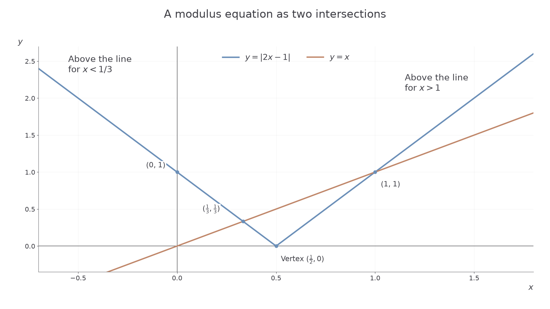
Keep the branch condition alongside each linear equation.

Worked example 3: solve a modulus equation

Question. Solve $|2x-1|=x$ .

Plan. Split at $x=\frac12$ , solve on both branches and check the branch restrictions.

\begin{aligned} x<\tfrac12:\quad 1-2x&=x &&\text{negative inner expression}\\ x&=\tfrac13 &&\text{collect terms}\\ x\ge\tfrac12:\quad 2x-1&=x &&\text{non-negative inner expression}\\ x&=1 &&\text{collect terms} \end{aligned}

Why check branches? A solution of a branch equation is valid only in the region where that branch describes the modulus.

Answer. $x=\frac13$ or $x=1$ , the two intersection inputs.

Check. $|\frac23-1|=\frac13$ and $|2-1|=1$ ; both inputs satisfy their branch conditions.

Change only the relation, from equality to “greater than”. The same intersections become boundary points.

Worked example 4: read the inequality intervals

Question. Solve $|2x-1|>x$ .

Plan. Use the two intersections and decide where the V lies above the line.

\begin{aligned} x<\tfrac12:\quad 1-2x>x&\implies x<\tfrac13 &&\text{left branch}\\ x\ge\tfrac12:\quad 2x-1>x&\implies x>1 &&\text{right branch} \end{aligned}

Why use “or”? Either separate interval puts the modulus graph above the line.

Answer. $x<\frac13$ or $x>1$ .

Check. Inputs $0$ and $2$ work; input $\frac12$ does not. Equality at the boundaries is excluded.

Modulus does not mean “remove minus signs inside the expression”. Its sign decision applies to the whole expression.

Watch out

The wrong line $|2x-1|=2x+1$ fails, for example, at $x=1$ . Use $2x-1$ or $1-2x$ according to the sign of $2x-1$ .

Change the coefficient and constant, then use the same two-branch route.

Reciprocal graphs and asymptotes

For $y=\frac2x$ , inputs $1,10,100$ give outputs $2,0.2,0.02$ . The output approaches zero without reaching it. Near $x=0$ , its magnitude instead grows without bound.

Asymptote

An asymptote is a line that a curve approaches as an input tends to infinity or to an excluded value. A vertical asymptote describes unbounded behaviour near an input; a horizontal asymptote describes a limiting height as $x\to\infty$ or $x\to-\infty$ .

The graphs $\frac ax$ and $\frac a{x^2}$ , $a\ne0$ , have asymptotes $x=0$ and $y=0$ . For $a>0$ , $\frac ax$ has opposite-sign branches, while $\frac a{x^2}$ has two positive branches. Negative $a$ reflects each graph in the horizontal axis.

[DIAGRAM: asset_name: Reciprocal shapes and translated asymptotes; asset_slug: p1_2_7_understand_and_use_graphs_of_functions_including_functions_defined_by_simple_polynomials_and_the_modulus_graph__diagram_03; caption: Denominator zeros locate vertical asymptotes; description: Three panels show y=2/x, y=2/x squared and y=2/(x+1)+1 with the last graph's asymptotes x=-1 and y=1.]

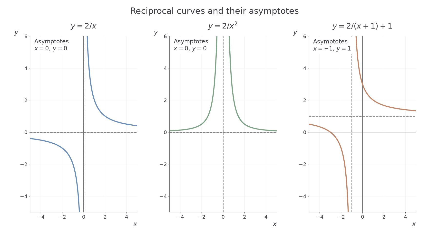
Translations move the limiting lines along with the curve.

Translated reciprocal graphs

For $a\ne0$ , each of

y=\frac a{x+p}+q,\qquad y=\frac a{(x+p)^2}+q

has asymptotes $x=-p$ and $y=q$ , with domain $x\ne-p$ .

Not in the formula booklet: learn it.

The first form changes sign relative to the height $q$ across its vertical asymptote; the squared form does not.

Worked example 5: translated reciprocal

Question. State the asymptotes and branch positions of $y=\frac3{x+2}-1$ .

Plan. Set the denominator to zero and inspect the fraction's sign relative to the limiting height.

\begin{aligned} x+2=0&\implies x=-2 &&\text{vertical asymptote}\\ \frac3{x+2}\to0&\implies y\to-1 &&\text{horizontal asymptote}\\ x>-2&\implies y>-1 &&\text{positive denominator}\\ x<-2&\implies y<-1 &&\text{negative denominator} \end{aligned}

Why compare with $-1$ ? The fraction measures the curve's height above or below that translated asymptote.

Answer. Asymptotes $x=-2$ , $y=-1$ ; branches lie upper-right and lower-left relative to $(-2,-1)$ .

Check. At $x=1$ , $y=0$ ; at $x=-5$ , $y=-2$ , agreeing with those regions.

Change only the denominator's power to $2$ . The limiting lines stay fixed, but the negative-denominator region disappears.

Worked example 6: translated reciprocal square

Question. State the asymptotes and branch positions of $y=\frac3{(x+2)^2}-1$ .

Plan. Use the same denominator zero, then note that the square is positive on both sides.

\begin{aligned} (x+2)^2=0&\implies x=-2 &&\text{vertical asymptote}\\ \frac3{(x+2)^2}\to0&\implies y\to-1 &&\text{horizontal asymptote}\\ \frac3{(x+2)^2}>0&\implies y>-1 &&\text{for }x\ne-2 \end{aligned}

Why are both branches above the limiting line? A positive numerator divided by a non-zero square is positive.

Answer. Asymptotes $x=-2$ , $y=-1$ ; both branches lie above $y=-1$ .

Check. At $x=-1$ and $x=-3$ , $y=2$ , showing the symmetry about $x=-2$ .

An asymptote is a line, so name it with an equation.

Watch out

“The asymptotes are $-2$ and $-1$ ” does not identify the lines. Write $x=-2$ and $y=-1$ . A general curve may cross a horizontal asymptote; these reciprocal forms do not.

Change the numerator's sign and read its effect on branch position.

Intersections as solutions

The equation $f(x)=g(x)$ asks where two graphs have the same height at the same input. Its solutions are the horizontal coordinates of their intersection points. To give the full coordinates, substitute each input into either function.

[DIAGRAM: asset_name: Cubic and line intersections; asset_slug: p1_2_7_intersections; caption: Three solutions correspond to three meetings; description: The graphs y=x cubed minus 4x and y=x intersect at inputs negative square root of 5, zero and positive square root of 5.]

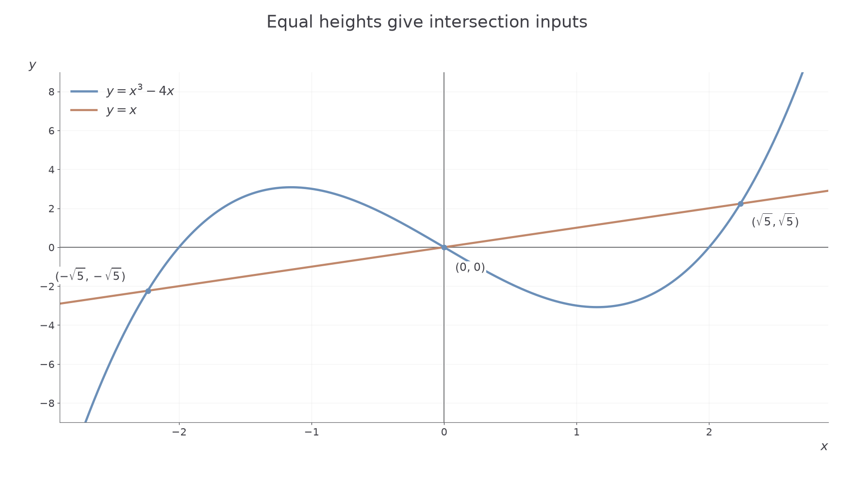
The graph predicts how many solutions to expect; algebra supplies their exact values.

Worked example 7: interpret a cubic equation

Question. Solve $x^3-4x=x$ and give a graphical interpretation.

Plan. Bring the heights to one side, then factorise.

\begin{aligned} x^3-5x&=0 &&\text{subtract }x\\ x(x^2-5)&=0 &&\text{factor out }x\\ x&=0,\ \pm\sqrt5 &&\text{zero-product rule} \end{aligned}

Why keep the factor $x$ ? Dividing by it would lose the zero solution.

Answer. $x=-\sqrt5,0,\sqrt5$ , the inputs where $y=x^3-4x$ meets $y=x$ .

Check. At $x=\sqrt5$ , $x^3-4x=5\sqrt5-4\sqrt5=\sqrt5$ .

Change only the line's gradient from $1$ to $2$ . The cubic stays fixed, but its intersection inputs move.

Worked example 8: move the intersecting line

Question. Find the coordinates where $y=x^3-4x$ meets $y=2x$ .

Plan. Equate the heights, factorise, then use the line for the vertical coordinates.

\begin{aligned} x^3-4x&=2x &&\text{equal heights}\\ x(x^2-6)&=0 &&\text{rearrange and factorise}\\ x&=0,\ \pm\sqrt6 &&\text{solve the factors}\\ y&=0,\ \pm2\sqrt6 &&\text{use }y=2x \end{aligned}

Why substitute back? Equation solutions alone give inputs, whereas intersection coordinates need both values.

Answer. $(-\sqrt6,-2\sqrt6)$ , $(0,0)$ , $(\sqrt6,2\sqrt6)$ .

Check. For $x=\sqrt6$ , the cubic gives $6\sqrt6-4\sqrt6=2\sqrt6$ .

Relative heights also explain inequalities: $f(x)>g(x)$ means the first graph is above the second, and $f(x)<g(x)$ means it is below.

Exam tip

Read the question carefully: “solve the equation” asks for inputs; “find the intersection points” asks for complete coordinate pairs.

Change the line's gradient once more.

Proportional relationships and their graphs

Proportion notation describes a constant multiple. If $C\propto d$ , then $C=kd$ for a constant $k$ ; doubling $d$ doubles $C$ . A straight-line graph through the origin records that constant ratio.

Proportional relationship

$y\propto F(x)$ means $y=kF(x)$ for a constant of proportionality $k$ . Direct proportion uses $F(x)=x$ ; inverse proportion uses $F(x)=\frac1x$ , with $x\ne0$ .

Other important forms are $y\propto x^2$ and $y\propto\frac1{x^2}$ . Their graphs are quadratic and reciprocal-square respectively. Their constants are found from $\frac y{x^2}=k$ and $yx^2=k$ . These relationships are not in the formula booklet: learn them.

[DIAGRAM: asset_name: Direct proportion versus a general linear relationship; asset_slug: p1_2_7_understand_and_use_graphs_of_functions_including_functions_defined_by_simple_polynomials_and_the_modulus_graph__diagram_04; caption: A constant ratio gives a line through the origin; description: The line y=2x passes through the origin; y=2x+3 does not and is not direct proportion.]

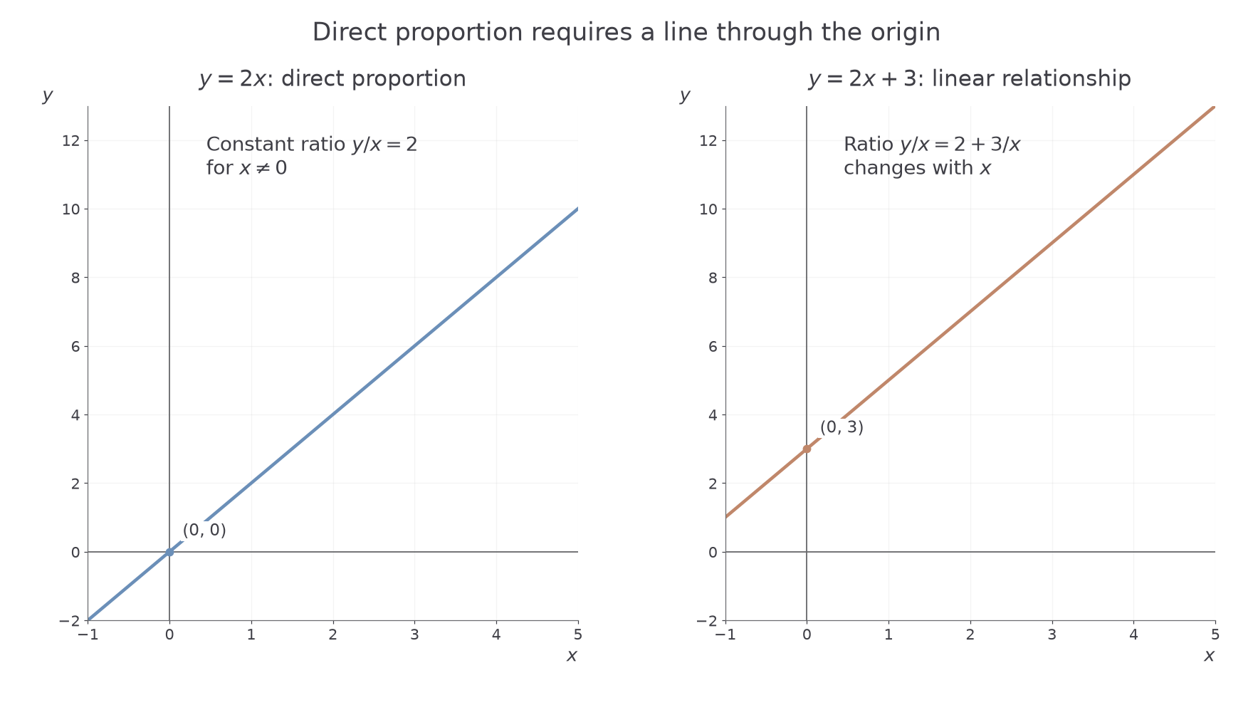
You can also linearise a power relationship: plotting $y$ against $x^2$ gives a straight line through the origin when $y=kx^2$ . Against $x$ , it is a parabola.

Worked example 9: direct proportion

Question. $C\propto d$ , and $C=20$ when $d=8$ . Find the relationship and describe its graph.

Plan. Replace the proportion sign by a constant multiplier and use the known pair.

\begin{aligned} C&=kd &&\text{direct proportion}\\ 20&=8k &&\text{substitute the pair}\\ k&=\tfrac52 &&\text{divide by }8 \end{aligned}

Why is the intercept zero? A constant multiple has no added fixed term.

Answer. $C=\frac52d$ , a straight line through the origin with gradient $\frac52$ .

Check. At $d=8$ , $C=\frac52(8)=20$ .

Change only the proportion law to inverse-square proportion, keeping the same known pair. The graph and the constant both change.

Worked example 10: inverse-square proportion

Question. $C\propto\frac1{d^2}$ , and $C=20$ when $d=8$ . Find the relationship and describe its graph for $d>0$ .

Plan. Write $C=\frac k{d^2}$ and multiply the known output by the square of its input.

\begin{aligned} 20&=\frac k{8^2} &&\text{substitute the pair}\\ k&=20(64)=1280 &&\text{multiply by }64\\ C&=\frac{1280}{d^2} &&\text{insert the constant} \end{aligned}

Why multiply rather than divide to find $k$ ? The invariant is $Cd^2$ , not $\frac C{d^2}$ .

Answer. $C=\frac{1280}{d^2}$ . For $d>0$ , it is the positive decreasing branch with asymptotes $d=0$ , $C=0$ .

Check. At $d=8$ , $C=20$ ; at $d=16$ , $C=5$ , a quarter as large.

For comparison, $y\propto\frac1x$ gives $y=\frac kx$ , and doubling a positive input halves the output. The inverse-square rule $y=\frac{48}{x^2}$ gives $y=12$ at $x=2$ ; it has the same shape as the new inverse-square model. A direct-square rule works the other way round: $P\propto x^2$ , with $P=27$ at $x=3$ , gives $k=27/9=3$ , so $P=3x^2$ .

Watch out

A linear graph need not show direct proportion: $y=3x+2$ is linear but $\frac yx=3+\frac2x$ is not constant. Check that the line passes through the origin.

Now change the known data for an inverse-square relationship.

Quick Recap

Read polynomial roots, multiplicities, intercepts and leading terms before drawing.
A linear modulus graph has two branches; intersections mark inequality boundaries.
Reciprocal denominator zeros give vertical asymptotes; vertical shifts give horizontal asymptotes.
Equation solutions are intersection inputs; full points need both coordinates.
Proportion means a constant multiple of the stated expression.

The opening quartic has two distinct double roots, so it touches twice and never crosses below the axis.

Last Accessed

Pure Mathematics (Papers 1 and 2)

Statistics (Paper 3, Section A)

Mechanics (Paper 3, Section B)

Pure 2.7 - Graphs of functions and the modulus graph

Sketching simple polynomial graphs

The modulus of a linear function

Reciprocal graphs and asymptotes

Intersections as solutions

Proportional relationships and their graphs

Quick Recap

Learn faster with Nova