Statistics 4.2 - Normal distribution as a model | Edexcel A-Level Mathematics

Use the Normal distribution to turn measurements into probabilities and probabilities back into unknown values. Connect its shape to data, recover its parameters, and approximate suitable Binomial counts with a continuity correction.

The Normal model and its shape

Why can a plant height and a component lifetime have exactly the same tail probability? Suppose plant height has mean $72\,\mathrm{cm}$ and standard deviation $4\,\mathrm{cm}$ , while component lifetime has mean $180$ hours and standard deviation $12$ hours. The values $78\,\mathrm{cm}$ and $198$ hours are each one and a half standard deviations above their own mean. A Normal model gives them the same upper-tail probability. We will find it shortly.

You already know

The mean describes the centre and the standard deviation describes spread. Variance is the square of standard deviation; probability from a density curve is area, rather than the curve's height.

A histogram with one approximately symmetric, bell-shaped mound suggests a Normal model. It does not prove the model: compare shape and context, including any impossible values near the centre.

Normal distribution

$X\sim N(\mu,\sigma^2)$ , with $\sigma>0$ , describes a continuous Normal variable with mean $\mu$ , variance $\sigma^2$ and standard deviation $\sigma$ . Its bell-shaped curve is symmetric about $x=\mu$ , has total area $1$ , and extends in both directions without meeting the horizontal axis.

Half the area lies on either side of the mean. Increasing $\sigma$ spreads the same area across a wider, lower curve; changing $\mu$ shifts the centre. A useful surprise is that every Normal distribution puts about $68.3\%$ of its probability within one standard deviation of its mean, regardless of the original units.

[DIAGRAM: asset_slug: p3_4_2_understand_and_use_the_normal_distribution_as_a_model__diagram_01; asset_name: Statistics 4.2 - Normal distribution as a model - diagram 01; description: A symmetric histogram suggesting a Normal model beside a Normal curve showing the mean, equal half-areas and inflection points one standard deviation either side.]
Diagram

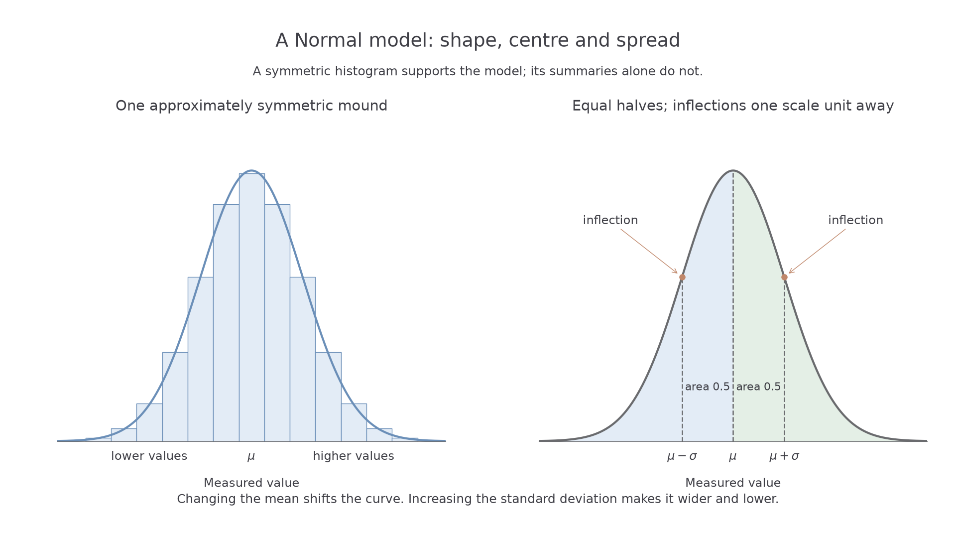
The changes of curvature give another link between the picture and its parameters.

Normal inflection points

For $X\sim N(\mu,\sigma^2)$ , the curve has points of inflection at

x=\mu-\sigma,\qquad x=\mu+\sigma.

Not in the formula booklet: learn it.

For the plants, $H\sim N(72,4^2)$ , so the inflection points are $68\,\mathrm{cm}$ and $76\,\mathrm{cm}$ , and $P(H>72)=0.5$ . For packaged masses $M\sim N(500,15^2)$ , the corresponding points are $485\,\mathrm g$ and $515\,\mathrm g$ . These use the standard deviation, rather than the second parameter itself. You need the inflection result, not its derivation or the Normal density formula.

Key idea

The first Normal parameter locates the centre; the square root of the second sets the scale.

Read the notation carefully before deciding where the curve changes curvature.

Finding Normal probabilities

A boundary becomes easier to interpret when you measure its distance from the mean in standard deviations. A value below the mean gives a negative standardised value; a value above it gives a positive one.

Standardising a Normal variable

If $X\sim N(\mu,\sigma^2)$ , with $\sigma>0$ , then

Z=\frac{X-\mu}{\sigma}\sim N(0,1).

Not in the formula booklet: learn it.

A calculator can find a probability directly using the original mean and standard deviation, or after standardisation using $N(0,1)$ . Both describe the same shaded area. The booklet supplies Normal percentage-point tables; its printed sample-mean formula is a different result.

[DIAGRAM: asset_slug: p3_4_2_understand_and_use_the_normal_distribution_as_a_model__diagram_02; asset_name: Statistics 4.2 - Normal distribution as a model - diagram 02; description: The same shaded interval shown on an original Normal scale and its standardised scale, with both endpoints transformed by subtracting the mean and dividing by the standard deviation.]
Diagram

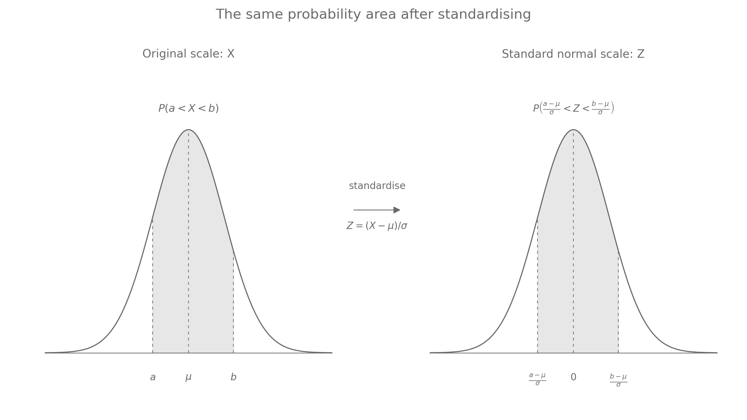
For a continuous Normal variable, $P(X=a)=0$ . Consequently $P(X<a)=P(X\le a)$ . There is no continuity correction when the variable is already a continuous measurement.

Worked example 1: an upper tail

Question. A component's lifetime satisfies $T\sim N(180,12^2)$ , in hours. Find $P(T>198)$ to three significant figures.

Plan. Standardise the cutoff and find the area to its right.

\begin{aligned} z&=\frac{198-180}{12}=1.5 &&\text{use the standard deviation}\\ P(T>198)&=P(Z>1.5) &&\text{preserve the required tail}\\ &=1-P(Z<1.5) &&\text{remove the left area}\\ &=0.0668072\ldots &&\text{evaluate with the calculator} \end{aligned}

Why subtract from $1$ ? The requested lifetimes are longer than the cutoff, whereas a left-tail function returns shorter lifetimes.

Answer. $P(T>198)=0.0668$ , so about $6.68\%$ exceed $198$ hours under the model.

Check. The cutoff is above the mean, so the upper-tail probability should be less than $0.5$ .

Change only the event: retain the same upper cutoff, but now include lifetimes from the equally distant lower cutoff up to it.

Worked example 2: a central interval

Question. For $T\sim N(180,12^2)$ , find $P(162<T<198)$ to three significant figures.

Plan. Transform both endpoints, then subtract their cumulative probabilities.

\begin{aligned} \frac{162-180}{12}&=-1.5,\qquad \frac{198-180}{12}=1.5 &&\text{standardise the boundaries}\\ P(162<T<198)&=P(-1.5<Z<1.5) &&\text{keep the interval}\\ &=P(Z<1.5)-P(Z<-1.5) &&\text{subtract the lower tail}\\ &=0.866385\ldots &&\text{evaluate the area} \end{aligned}

Why subtract the lower cumulative value? It removes the outcomes below $162$ that the upper cumulative value includes.

Answer. $P(162<T<198)=0.866$ .

Check. Symmetry gives $1-2(0.0668072\ldots)=0.866385\ldots$ , agreeing with the direct calculation.

The boundaries need not be symmetric. For $X\sim N(65,8^2)$ ,

P(60<X<72)=P(-0.625<Z<0.875)=0.543227\ldots.

The calculator still needs both endpoints and the standard deviation $8$ .

Watch out

For $N(65,8^2)$ , entering standard deviation $64$ changes the model. Enter $8$ , and write the probability statement before calculating.

Keep the central-interval method, but move the lower boundary.

Working backwards from probabilities

If a probability is given, inverse Normal finds the boundary on the standard scale. You can then recover a cutoff, mean or standard deviation by rearranging the standardisation equation.

An inverse Normal equation

For $X\sim N(\mu,\sigma^2)$ and $0<q<1$ , let $z_q$ satisfy $P(Z<z_q)=q$ . Then

P(X<c)=q\quad\Longrightarrow\quad c=\mu+z_q\sigma.

Not in the formula booklet: learn it.

Convert a right-tail probability into a left-tail probability first if that is what your calculator requests. Sketch the cutoff relative to the mean to predict the sign of $z_q$ .

Worked example 3: an unknown standard deviation

Question. $X\sim N(100,\sigma^2)$ and $P(X>112)=0.08$ . Find $\sigma$ to three significant figures.

Plan. Convert the tail, find its inverse Normal value and solve for the positive standard deviation.

\begin{aligned} P(X<112)&=0.92 &&\text{take the complement}\\ z_{0.92}&=1.405071\ldots &&\text{inverse Normal}\\ \frac{112-100}{\sigma}&=1.405071\ldots &&\text{standardise the cutoff}\\ \sigma&=\frac{12}{1.405071\ldots}=8.54049\ldots &&\text{solve without rounding early} \end{aligned}

Why is the $z$ -value positive? The cutoff $112$ is above the mean $100$ .

Answer. $\sigma=8.54$ .

Check. Substituting the unrounded value into $P(X>112)$ returns $0.08$ ; $\sigma$ is positive as required.

Change only the right-tail probability from $0.08$ to $0.10$ . A larger tail beyond the same cutoff needs a larger spread.

Worked example 4: changing the tail size

Question. $X\sim N(100,\sigma^2)$ and $P(X>112)=0.10$ . Find $\sigma$ to three significant figures.

Plan. Repeat the inverse Normal equation with the new left-tail area.

\begin{aligned} P(X<112)&=0.90 &&\text{convert to a left tail}\\ z_{0.90}&=1.281551\ldots &&\text{inverse Normal}\\ 12&=1.281551\ldots\sigma &&\text{rearrange standardisation}\\ \sigma&=9.36364\ldots &&\text{divide by the unrounded value} \end{aligned}

Why has the spread increased? The model must put more area beyond a fixed distance above its mean.

Answer. $\sigma=9.36$ .

Check. It exceeds $8.54$ , matching that prediction, and gives the specified $0.10$ upper tail.

If the unknown is the mean instead, rearrange to $\mu=c-z_q\sigma$ . For example, $X\sim N(\mu,4^2)$ with $P(X<58)=0.90$ gives

58=\mu+1.281551\ldots(4)\quad\Rightarrow\quad \mu=52.8737\ldots.

If both parameters are known, the same equation finds the percentile $c$ . Do not substitute the probability $0.90$ where its inverse Normal value belongs.

Watch out

A lower-tail area below $0.5$ gives a negative $z$ -value. A calculated negative standard deviation signals a sign or tail error; it is not an acceptable solution.

Increase the right-tail probability once more, keeping the same mean and cutoff.

Finding both Normal parameters

Two unknown parameters need two independent pieces of information. Two known cumulative probabilities produce two linear equations in $\mu$ and $\sigma$ .

Keep inverse Normal values unrounded in the calculator; when quoting them, at least four decimal places usually matches the tables' precision. Show the equations and a visible elimination step, so a small earlier error does not hide the method.

Continue this lesson.

You’re previewing NovaLearn without an account. Create a free account to read the rest.

Create free account

Last Accessed

Pure Mathematics (Papers 1 and 2)

Statistics (Paper 3, Section A)

Mechanics (Paper 3, Section B)

Statistics 4.2 - Normal distribution as a model

The Normal model and its shape

Finding Normal probabilities

Working backwards from probabilities

Finding both Normal parameters

Continue this lesson.

Learn faster with Nova