Pure 2.9 - Transformations of functions | Edexcel A-Level Mathematics

A graph can move, stretch, reflect or fold without losing its connection to the original function. Learn to track key points and asymptotes through those changes, then sketch combinations for polynomial, reciprocal, trigonometric and exponential functions.

The point-mapping idea

A curve passes through $(4,-3)$ . Where does that point go on $y=3f(-x)+5$ ? You can answer even if nobody tells you the formula for $f$ . The old input must still reach $4$ ; then the old height $-3$ is multiplied by $3$ and increased by $5$ .

You already know

If $(p,q)$ lies on $y=f(x)$ , then $f(p)=q$ . Substitution inside $f$ changes its input; operations outside $f$ change its output.

Solve for the new horizontal coordinate by making the new inner expression equal the old input. Then apply the outside operation to the old height.

Basic point mappings

For a point $(p,q)$ on $y=f(x)$ ,

\begin{array}{c|c} \text{new graph}&\text{new point}\\\hline y=f(x)+a&(p,q+a)\\ y=af(x)&(p,aq)\\ y=f(x+a)&(p-a,q)\\ y=f(ax)&(p/a,q),\quad a\ne0 \end{array}

Not in the formula booklet: learn it.

The inside changes can feel backwards. An equation for the input explains them more reliably than a memory trick.

Worked example 1: shift an input

Question. $P(4,-3)$ lies on $y=f(x)$ . Find its image on $y=f(x-2)$ .

Plan. Make $x-2$ equal the old input and keep the output unchanged.

\begin{aligned} x-2&=4 &&\text{match the old input}\\ x&=6 &&\text{solve}\\ y&=-3 &&\text{no outside change} \end{aligned}

Why move right? The new input must be $2$ larger to compensate for subtracting $2$ inside.

Answer. $P\mapsto(6,-3)$ .

Check. At the new input $6$ , the function receives $6-2=4$ , giving $-3$ .

Change only the sign of the inside constant, from $-2$ to $+2$ . The direction of the shift reverses.

Worked example 2: reverse the horizontal shift

Question. Find the image of $P(4,-3)$ on $y=f(x+2)$ .

Plan. Set the new inner input equal to $4$ .

\begin{aligned} x+2&=4 &&\text{same old input}\\ x&=2 &&\text{solve}\\ y&=-3 &&\text{same old height} \end{aligned}

Why does adding inside move left? A smaller new input reaches the original input after $2$ is added.

Answer. $P\mapsto(2,-3)$ .

Check. $f(2+2)=f(4)=-3$ .

These are point images on a new graph; they do not claim the original graph also contains those new points.

Watch out

For $f(x+2)$ , the wrong image $(6,-3)$ confuses inside and outside changes. Solve $x+2=4$ to obtain $(2,-3)$ .

Change the original point and the inside shift for your turn.

Translations and stretches

A translation adds the same displacement to every point. A stretch multiplies distances from an axis by a fixed positive scale factor. A negative multiplier includes a reflection.

Rule	Geometric change
$f(x)+a$	translation by $\binom0a$
$f(x+a)$	translation by $\binom{-a}0$
$af(x)$ , $a\ne0$	stretch parallel to the vertical axis by $
$f(ax)$ , $a\ne0$	stretch parallel to the horizontal axis by $\frac1{

In particular, $-f(x)$ reflects in the horizontal axis and $f(-x)$ reflects in the vertical axis. If $a=0$ , $af(x)=0$ wherever $f$ is defined, while $f(ax)=f(0)$ if that value exists; neither is a reversible stretch.

[DIAGRAM: asset_name: Horizontal and vertical stretches; asset_slug: p1_2_9_understand_the_effect_of_simple_transformations_on_the_graph_of_y_f_x__diagram_01; caption: Horizontal coordinates divide by three and heights double; description: The parabola f(x)=one half x squared minus 2 and y=2f(3x) show mapped roots plus or minus 2 to plus or minus two thirds and vertex (0,-2) to (0,-4).]

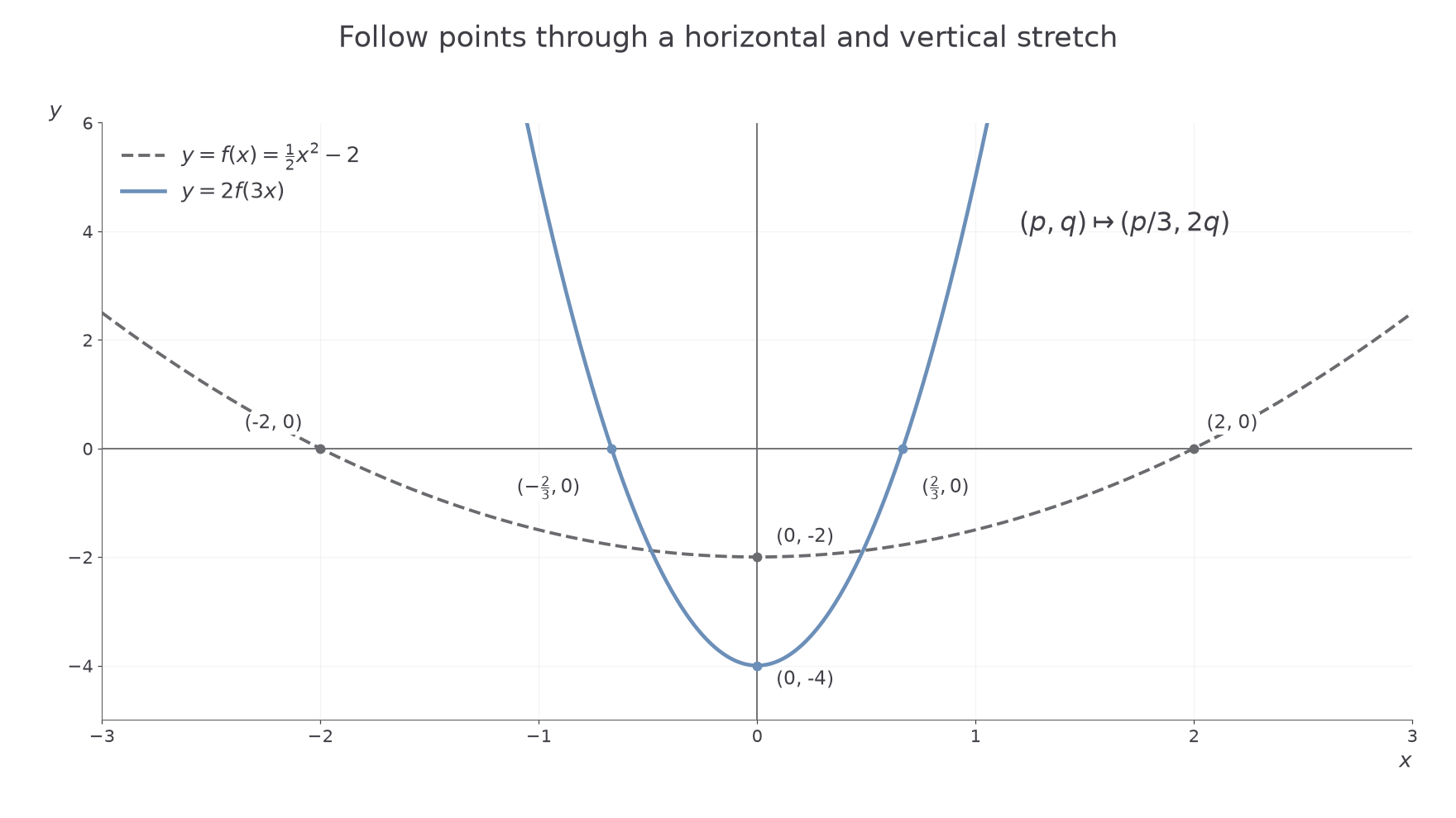
Distances from different axes change independently, so horizontal and vertical stretches can be followed together.

Worked example 3: stretch in both directions

Question. A graph has key points $(-3,1)$ , $(0,-1)$ , $(3,2)$ . Find their images on $y=2f(3x)$ .

Plan. Divide old inputs by $3$ and multiply old outputs by $2$ .

\begin{aligned} 3x=p&\implies x=p/3 &&\text{match the input}\\ y&=2q &&\text{double the height}\\ (-3,1)&\mapsto(-1,2)\\ (0,-1)&\mapsto(0,-2)\\ (3,2)&\mapsto(1,4) \end{aligned}

Why divide the inputs? Reaching the old input through $3x$ takes only one third of the horizontal coordinate.

Answer. The images are $(-1,2)$ , $(0,-2)$ , $(1,4)$ .

Check. At new input $1$ , the inner input is $3$ , whose old output $2$ becomes $4$ .

Change only the vertical multiplier from $2$ to $-2$ . The horizontal stretch stays fixed, and reflection reverses all heights.

Worked example 4: include a reflection

Question. Find the images of the same points on $y=-2f(3x)$ .

Plan. Keep the horizontal rule and negate the doubled outputs.

\begin{aligned} (p,q)&\mapsto(p/3,-2q) &&\text{combined stretch and reflection}\\ (-3,1)&\mapsto(-1,-2)\\ (0,-1)&\mapsto(0,2)\\ (3,2)&\mapsto(1,-4) \end{aligned}

Why does a maximum become a minimum? Multiplying heights by a negative number reverses their order.

Answer. $(-1,-2)$ , $(0,2)$ , $(1,-4)$ .

Check. Reflecting the previous three images in the horizontal axis gives precisely these points.

Translations can be combined too: $(-4,6)$ becomes $(-2,9)$ on $f(x-2)+3$ , since $x-2=-4$ and $y=6+3$ .

Exam tip

Name a stretch's direction and scale factor. For $f(3x)$ , the horizontal scale factor is $\frac13$ , not $3$ .

Change the vertical multiplier once more while retaining the horizontal rule.

Modulus graphs

Taking the modulus of an output folds negative heights upwards. It leaves positive heights and all roots fixed. If an original curve crosses the axis, its folded graph often has a corner there.

Modulus point mappings

For $(p,q)$ on $y=f(x)$ ,

y=|f(x)|:\ (p,q)\mapsto(p,|q|),\qquad y=|f(-x)|:\ (p,q)\mapsto(-p,|q|).

The first rule changes outputs; the second also reflects inputs.

Not in the formula booklet: learn it.

For $|f(-x)|$ , reflect in the vertical axis, then fold negative heights above the horizontal axis.

[DIAGRAM: asset_name: Modulus folds and reflection; asset_slug: p1_2_9_understand_the_effect_of_simple_transformations_on_the_graph_of_y_f_x__diagram_02; caption: Fold negative outputs upwards, then track the horizontal reflection; description: The quadratic f(x)=(x-1) squared divided by 3 minus 3 has roots -2 and 4 and minimum (1,-3). Panels compare it with absolute value f(x), and show absolute value f(-x) with roots -4 and 2 and image (-1,3).]

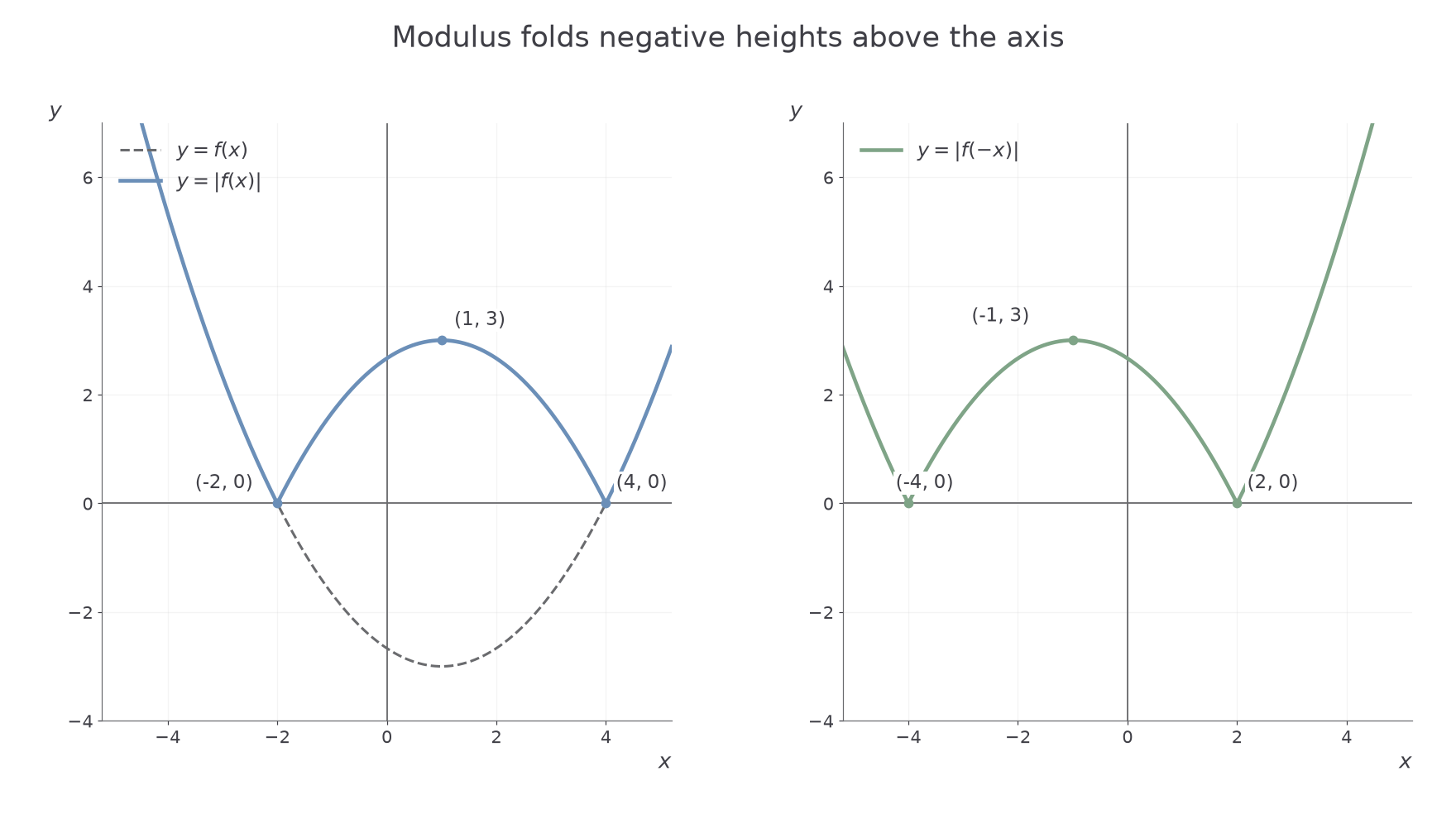
The minimum's image in the negative region becomes a local maximum after folding, even though its height becomes positive.

Worked example 5: fold a graph above the axis

Question. A graph has roots $-2,4$ and minimum $(1,-3)$ . Find the corresponding features of $y=|f(x)|$ .

Plan. Keep inputs and replace each output by its modulus.

\begin{aligned} (-2,0)&\mapsto(-2,0) &&\text{zero stays zero}\\ (4,0)&\mapsto(4,0) &&\text{zero stays zero}\\ (1,-3)&\mapsto(1,3) &&\text{reflect the negative height} \end{aligned}

Why keep the roots? Taking modulus cannot change a zero into a positive number.

Answer. Roots remain $-2,4$ ; the old minimum maps to the local maximum $(1,3)$ .

Check. Every transformed height is non-negative, including $|-3|=3$ .

Change only the input from $x$ to $-x$ . The fold stays the same; the horizontal coordinates reverse signs.

Worked example 6: reflect and fold

Question. For the same original graph, find the corresponding features of $y=|f(-x)|$ .

Plan. Negate the input coordinates and take the modulus of the output coordinates.

\begin{aligned} (-2,0)&\mapsto(2,0) &&\text{reflect the input}\\ (4,0)&\mapsto(-4,0) &&\text{reflect the input}\\ (1,-3)&\mapsto(-1,3) &&\text{reflect and fold} \end{aligned}

Why does the root at $4$ move to $-4$ ? The new inner input must satisfy $-x=4$ .

Answer. Roots $-4,2$ , and local maximum $(-1,3)$ .

Check. At $x=-1$ , $|f(-x)|=|f(1)|=|-3|=3$ .

A graph defined only on a restricted domain also has its domain reflected when $x$ becomes $-x$ .

Watch out

$|f(x)|$ changes outputs; $f(|x|)$ changes inputs. These are different instructions. For this lesson, the required folds are $|f(x)|$ and $|f(-x)|$ .

Use new point and root data with the reflected modulus rule.

Combining transformations

When a shift and stretch occur in the same direction, their order matters. One combined point rule avoids guessing the order. Set the complete inner expression equal to the old input before changing the output.

Combined point rule

If $(p,q)$ lies on $y=f(x)$ , then for $A\ne0$ , $B\ne0$ ,

y=Af(Bx+C)+D:\qquad(p,q)\mapsto\left(\frac{p-C}{B},Aq+D\right).

The rule also maps the positions of vertical and horizontal asymptotes; those lines are not points on the curve.

Not in the formula booklet: learn it.

For instance, $f(2x-2)=f(2(x-1))$ can be obtained by a horizontal stretch of scale factor $\frac12$ , followed by translation right $1$ . Translating right $1$ first and then stretching gives $f(2x-1)$ , a different graph.

Worked example 7: transform two turning points

Question. The graph of $f$ has maximum $(-1,3)$ and minimum $(4,-2)$ . Find their images on $y=-2f(2x-1)+3$ .

Plan. Solve $2x-1=p$ and use $y=-2q+3$ .

\begin{aligned} x&=(p+1)/2 &&\text{solve the inner equation}\\ (-1,3)&\mapsto(0,-3) &&\text{insert both coordinates}\\ (4,-2)&\mapsto(5/2,7) &&\text{insert both coordinates} \end{aligned}

Why do the turning-point types swap? The negative outside multiplier reverses vertical order.

Answer. Minimum $(0,-3)$ and maximum $(\frac52,7)$ .

Check. At new input $0$ , the old input is $-1$ , and $-2(3)+3=-3$ .

Change only the outside shift from $+3$ to $-1$ . Both image heights move down by $4$ , while their inputs stay fixed.

Worked example 8: alter the final translation

Question. Find those turning-point images on $y=-2f(2x-1)-1$ .

Plan. Retain $x=(p+1)/2$ and replace the output rule by $-2q-1$ .

\begin{aligned} (-1,3)&\mapsto\left(0,-2(3)-1\right)=(0,-7)\\ (4,-2)&\mapsto\left(5/2,-2(-2)-1\right)=(5/2,3) \end{aligned}

Why does the horizontal position stay fixed? Only the outside constant changed.

Answer. Minimum $(0,-7)$ and maximum $(\frac52,3)$ .

Check. Both outputs are $4$ lower than in the preceding example, as expected.

Apply exactly the same equations to asymptotes. If the original has $x=4$ , $y=-2$ , then $-2f(2x-1)+3$ has asymptotes $x=\frac52$ , $y=7$ .

Problem-solving

Use the equation $Bx+C=p$ , rather than multiplying the old horizontal coordinate by $B$ . This works for roots, endpoints and asymptote positions too.

Change the final output shift with fresh point data.

Named function sketches

The point rule works for every function family in this course. You only need to choose the features that carry its shape. Trigonometric angles below are in radians; later trigonometry lessons develop those base curves in detail.

Base family	Features to transform
quadratic, cubic, quartic	roots, vertical intercept, turning points, distant ends
$a/x$ , $a/x^2$	vertical and horizontal asymptotes, branch signs
sine and cosine	midline, amplitude, period, maxima and minima
tangent	roots, period and vertical asymptotes
$e^x$ , $a^x$ , $a>0,a\ne1$	$(0,1)$ , limiting height zero and growth or decay direction

For example, $(x-1)^2+2$ has vertex $(1,2)$ ; $(x-1)^3+2$ has its flattened crossing of height $2$ there; $(x-1)^4+2$ has a minimum there. Each comes from translating its power graph right $1$ , up $2$ . Likewise, $\frac1{x-1}+2$ and $\frac1{(x-1)^2}+2$ have asymptotes $x=1$ , $y=2$ .

[DIAGRAM: asset_name: Transformed sine and cosine; asset_slug: p1_2_9_understand_the_effect_of_simple_transformations_on_the_graph_of_y_f_x__diagram_03; caption: Changing sine to cosine shifts the key points but preserves range and period; description: Two panels show y=3+sin(2x) and y=3+cos(2x) for 0 to 2pi, each with midline 3, period pi and range 2 to 4.]

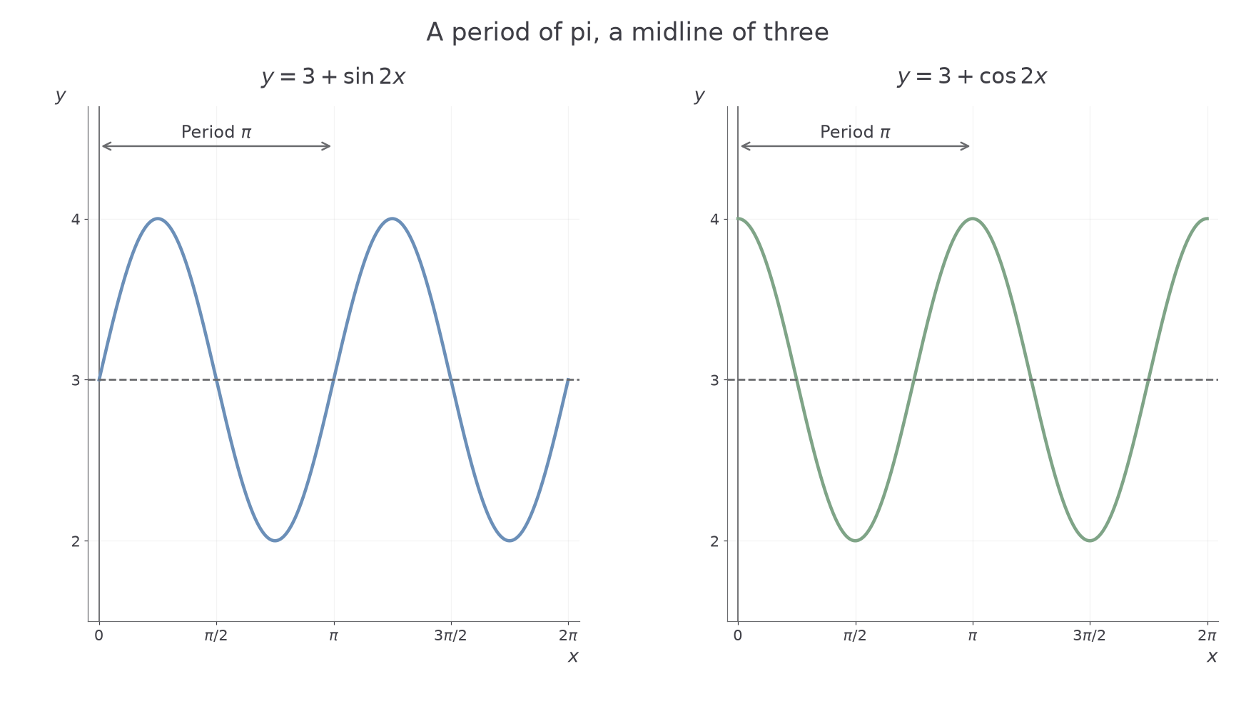
For a sine or cosine curve, a horizontal scale factor of $\frac1{|B|}$ changes its period from $2\pi$ to $\frac{2\pi}{|B|}$ . This transformation result is not in the formula booklet: learn it.

Worked example 9: transform a sine graph

Question. Give the features needed to sketch $y=3+\sin2x$ , $0\le x\le2\pi$ .

Plan. Transform one sine cycle, then repeat it with its new period.

\begin{aligned} \text{period}&=2\pi/2=\pi &&\text{horizontal scale }1/2\\ -1\le\sin2x\le1&\implies2\le y\le4 &&\text{add }3\\ 2x=\pi/2+2k\pi&\implies x=\pi/4+k\pi &&\text{maximum inputs}\\ 2x=3\pi/2+2k\pi&\implies x=3\pi/4+k\pi &&\text{minimum inputs} \end{aligned}

Why find key heights first? They give an unambiguous wave without plotting many points.

Answer. Midline $y=3$ , amplitude $1$ , period $\pi$ ; maxima $(\frac\pi4,4)$ , $(\frac{5\pi}4,4)$ ; minima $(\frac{3\pi}4,2)$ , $(\frac{7\pi}4,2)$ ; starts at $(0,3)$ rising.

Check. At $x=\frac\pi4$ , $y=3+\sin\frac\pi2=4$ ; at $x=\pi$ , $y=3$ , one cycle later.

Change only the base function from sine to cosine. The stretch and translation stay the same.

Worked example 10: transform a cosine graph

Question. Give the features needed to sketch $y=3+\cos2x$ , $0\le x\le2\pi$ .

Plan. Keep the range and period, then track cosine's maxima and minima.

\begin{aligned} \text{period}&=\pi &&\text{same horizontal stretch}\\ 2\le y&\le4 &&\text{same vertical translation}\\ 2x=2k\pi&\implies x=k\pi &&\text{maxima}\\ 2x=\pi+2k\pi&\implies x=\pi/2+k\pi &&\text{minima} \end{aligned}

Why does it start at a maximum? $\cos0=1$ , whereas $\sin0=0$ .

Answer. Midline $3$ , amplitude $1$ , period $\pi$ ; maxima at $x=0,\pi,2\pi$ , height $4$ ; minima at $x=\frac\pi2,\frac{3\pi}2$ , height $2$ .

Check. $y(0)=4$ and $y(\frac\pi2)=3+\cos\pi=2$ .

Other families use the same reasoning. The graph $-\cos(x+\frac\pi4)$ shifts cosine left $\frac\pi4$ and reflects it in the horizontal axis; its minimum is $(-\frac\pi4,-1)$ . The graph $\tan2x$ has period $\frac\pi2$ , roots $x=\frac{k\pi}2$ and asymptotes $x=\frac\pi4+\frac{k\pi}2$ , where $k\in\mathbb Z$ .

Exponential graphs transform too: $2e^{-x}+1$ reflects $e^x$ in the vertical axis, doubles heights and shifts up $1$ , giving $(0,3)$ and horizontal asymptote $y=1$ . Replacing $e^x$ by $2^x$ gives $2\cdot2^{-x}+1$ , with the same intercept and limiting height. A surprising contrast: for reciprocal curves $2f(3x)=\frac23f(x)$ when $f(x)=\frac1x$ , but for $f(x)=\frac1{x^2}$ it is $\frac29f(x)$ . The same geometric instruction can simplify differently for different families.

The opening point now follows immediately: $-x=4$ gives $x=-4$ , and $3(-3)+5=-4$ , so it moves to $(-4,-4)$ .

Exam tip

On a sketch, label the transformed features that distinguish the curve: a period and height for a wave, or asymptotes and an intercept for a reciprocal or exponential graph.

Keep cosine and change the input multiplier for the final check.

Quick Recap

Outside operations change heights; inside operations require solving for the new input.
Negative multipliers introduce reflections; inside stretch factors act reciprocally on coordinates.
Modulus folds negative heights upwards; $|f(-x)|$ also reflects horizontally.
A combined graph maps $(p,q)$ to $(\frac{p-C}B,Aq+D)$ .
Track the defining features of each function family.

The opening point $(4,-3)$ becomes $(-4,-4)$ on $y=3f(-x)+5$ , without needing a formula for $f$ .

Last Accessed

Pure Mathematics (Papers 1 and 2)

Statistics (Paper 3, Section A)

Mechanics (Paper 3, Section B)

Pure 2.9 - Transformations of functions

The point-mapping idea

Translations and stretches

Modulus graphs

Combining transformations

Named function sketches

Quick Recap

Learn faster with Nova