Statistics 3.3 - Probability modelling and assumptions

Probability models and assumptions

If a coin is slightly more likely to land heads, does every familiar fair-coin prediction become larger? Start with four tosses: the fair independent model gives $16$ equally likely sequences, and $5$ contain at least three heads. We will change the assumption and see which predictions rise and which fall.

A model is a deliberate simplification, rather than a claim that every detail of the world has been captured.

Fairness means equally likely outcomes: for a coin $P(H)=P(T)=1/2$, while for a fair die every face has probability $1/6$. Independence is a separate assumption about how trials relate. A fair coin need not produce independent results in a badly designed experiment.

[DIAGRAM: asset_slug: p3_3_3_understand_and_model_with_probability_including_critiquing_assumptions__diagram_01; asset_name: Statistics 3.3 - Probability modelling and assumptions - diagram 01; caption: Predictions feed back into assumptions through evidence; description: The modelling cycle moves from real situation through assumptions, probability model, prediction, evidence and refinement.]

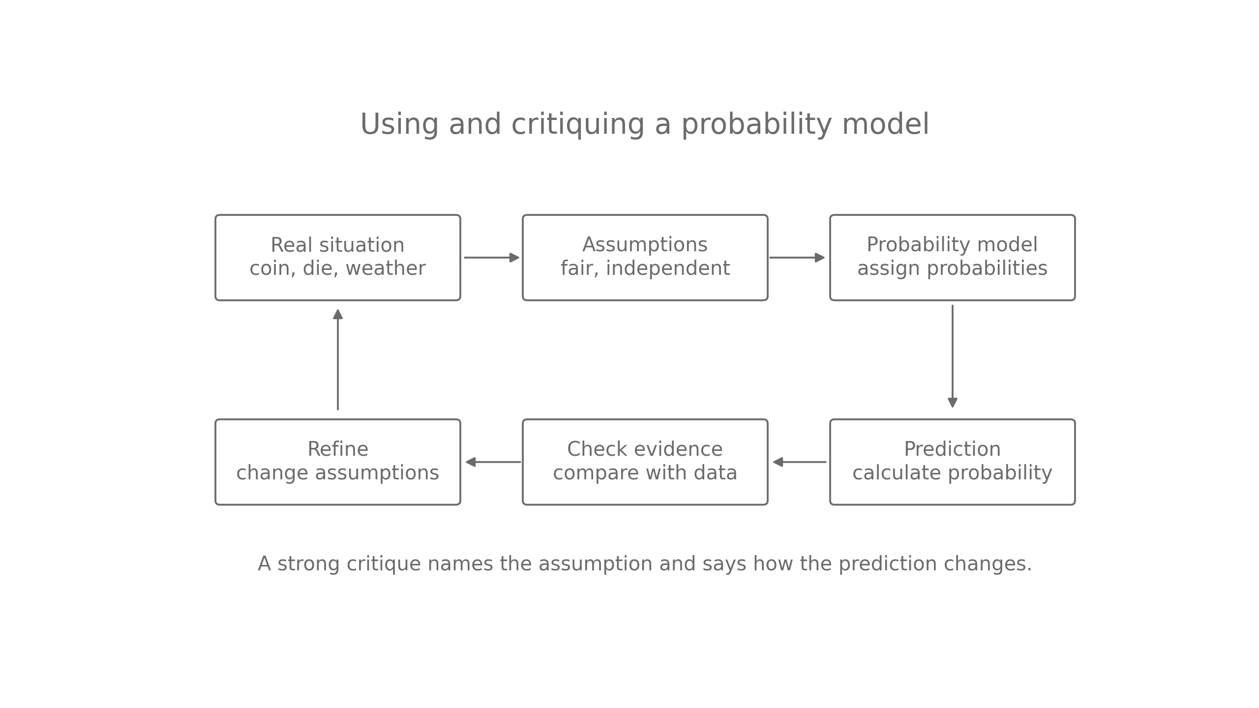
Construct the model, calculate under its assumptions, then judge what the result means.

Change only the probability of heads to $0.55$. Keep the tosses independent, so a path's probability still multiplies.

A four-sector fair spinner spun independently twice similarly gives $P(\text{two As})=(1/4)^2=1/16$. Equal sector probabilities and independence are distinct assumptions used at different steps.

Move the heads probability again, keeping all other features fixed.

Fair models and more realistic models

Fairness is convenient, but worn objects or the way they are used can favour some outcomes. A refined model changes the probabilities for a stated reason. It still has to satisfy the probability rules.

[DIAGRAM: asset_slug: p3_3_3_understand_and_model_with_probability_including_critiquing_assumptions__diagram_02; asset_name: Statistics 3.3 - Probability modelling and assumptions - diagram 02; caption: Increasing the six probability changes a two-roll prediction; description: A fair die has six probabilities of one sixth. A loaded model assigns 0.15 to each of faces one to five and 0.25 to six; the corresponding probabilities of two sixes are one thirty-sixth and one sixteenth.]

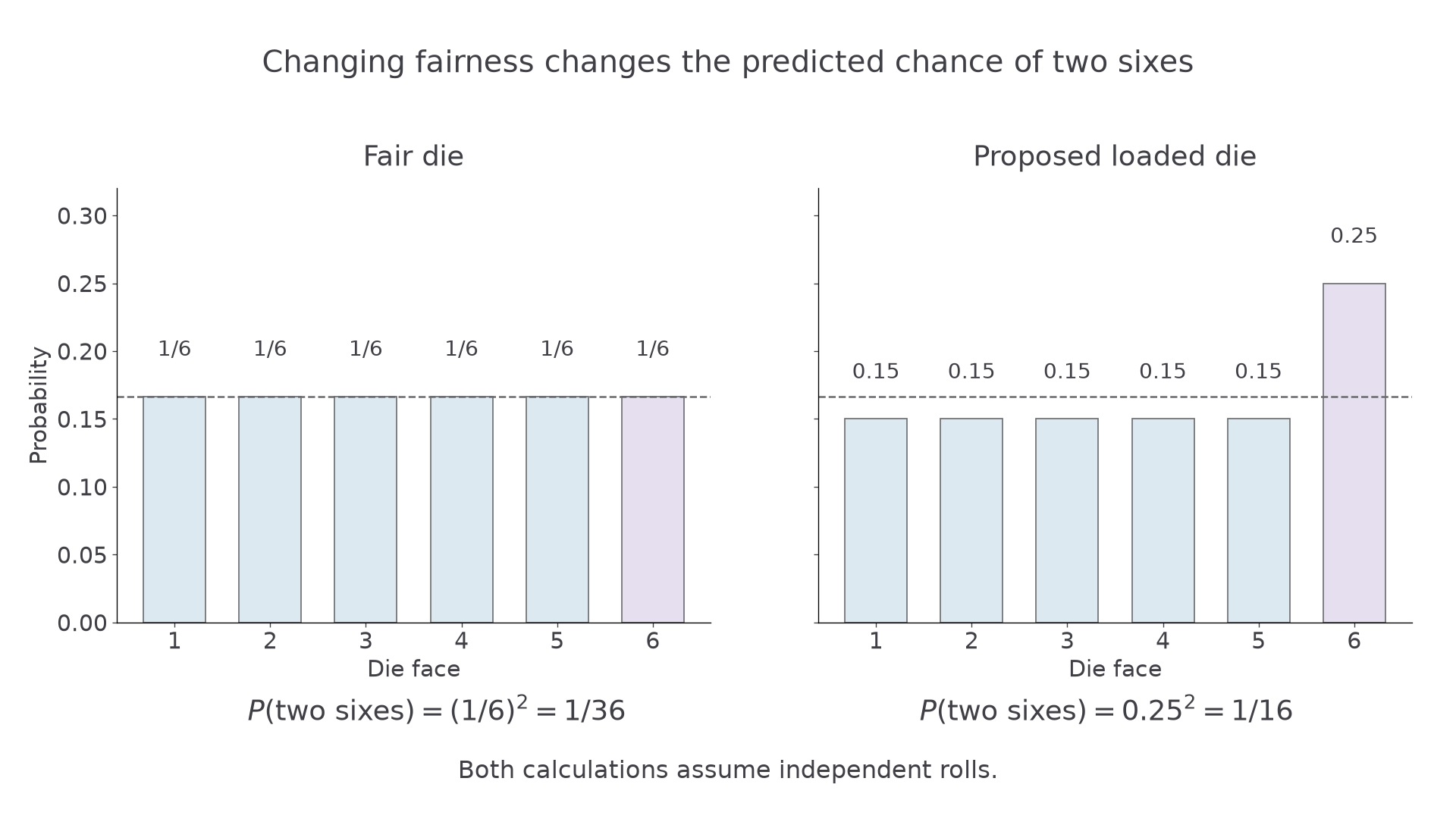
The loaded model is valid because $5(0.15)+0.25=1$, with all probabilities nonnegative. “More realistic” needs evidence about the particular die; these values describe a proposed model rather than measured data.

Change only $P(6)$ from $1/6$ to $0.25$, keeping independent rolls.

The direction of change depends on the event. Here is a useful surprise: for two independent coin tosses with $P(H)=p$,

With $p=0.50$ this is $0.50$, but with $p=0.55$ it is $0.495$. Favouring heads raises the chance of two heads while lowering the chance of exactly one. Likewise $P(H)=0.58$ gives two-head probability $0.3364$, above the fair value $0.25$.

Change only the proposed six probability once more.

Comparing a model with evidence

Observed data help judge a model, but a mismatch can arise through random variation. Comparing a relative frequency with a model probability is evidence, rather than a proof that the model is false.

Pearson's weather Large Data Set records daily mean cloud in oktas. At Heathrow in June 2015, the $30$ recorded values have these frequencies:

A proposed uniform model assigns probability $1/9$ to each integer $0,\ldots,8$. It is a useful model to question, rather than a claim that all cloud amounts really occur equally often.

Change only the event threshold from $4$ to $2$. Keep the same model and actual observations.