Statistics 4.1 - Discrete and binomial probability distributions | Edexcel A-Level Mathematics

Use a probability distribution to describe a whole set of possible outcomes. Build Binomial models, calculate individual and cumulative probabilities, and decide whether the assumptions fit the situation.

What a discrete distribution tells you

If a spinner has four possible scores, must each score have probability $\frac14$ ? A spinner with four equal sectors labelled $1$ , $2$ , $3$ and $4$ does. Change the sector sizes, and the same four scores can have quite different probabilities. The list of possible values is only half the story.

You already know

Probabilities lie between $0$ and $1$ . Mutually exclusive outcomes covering every possibility have probabilities adding to $1$ .

A capital letter names the random variable; a lower-case letter names a possible value. For example, $X$ is the score on a fair six-sided die, while $x=4$ is one possible score.

Discrete probability distribution

A discrete random variable takes separate countable values. Its probability distribution lists every possible value $x$ and its probability $P(X=x)$ , with

0\le P(X=x)\le1,\qquad \sum_x P(X=x)=1.

A discrete uniform distribution has equal probabilities for all its possible values.

The fair die has six probabilities of $\frac16$ . A distribution need not be uniform: the Binomial bars on the right have different heights because some counts can occur in more ways than others.

[DIAGRAM: asset_slug: p3_4_1_understand_and_use_simple_discrete_probability_distributions__diagram_01; asset_name: Statistics 4.1 - Discrete and binomial probability distributions - diagram 01; description: Equal-height probabilities for a fair six-sided die beside the unequal probabilities of a Binomial B(6, 0.4) count.]
Diagram

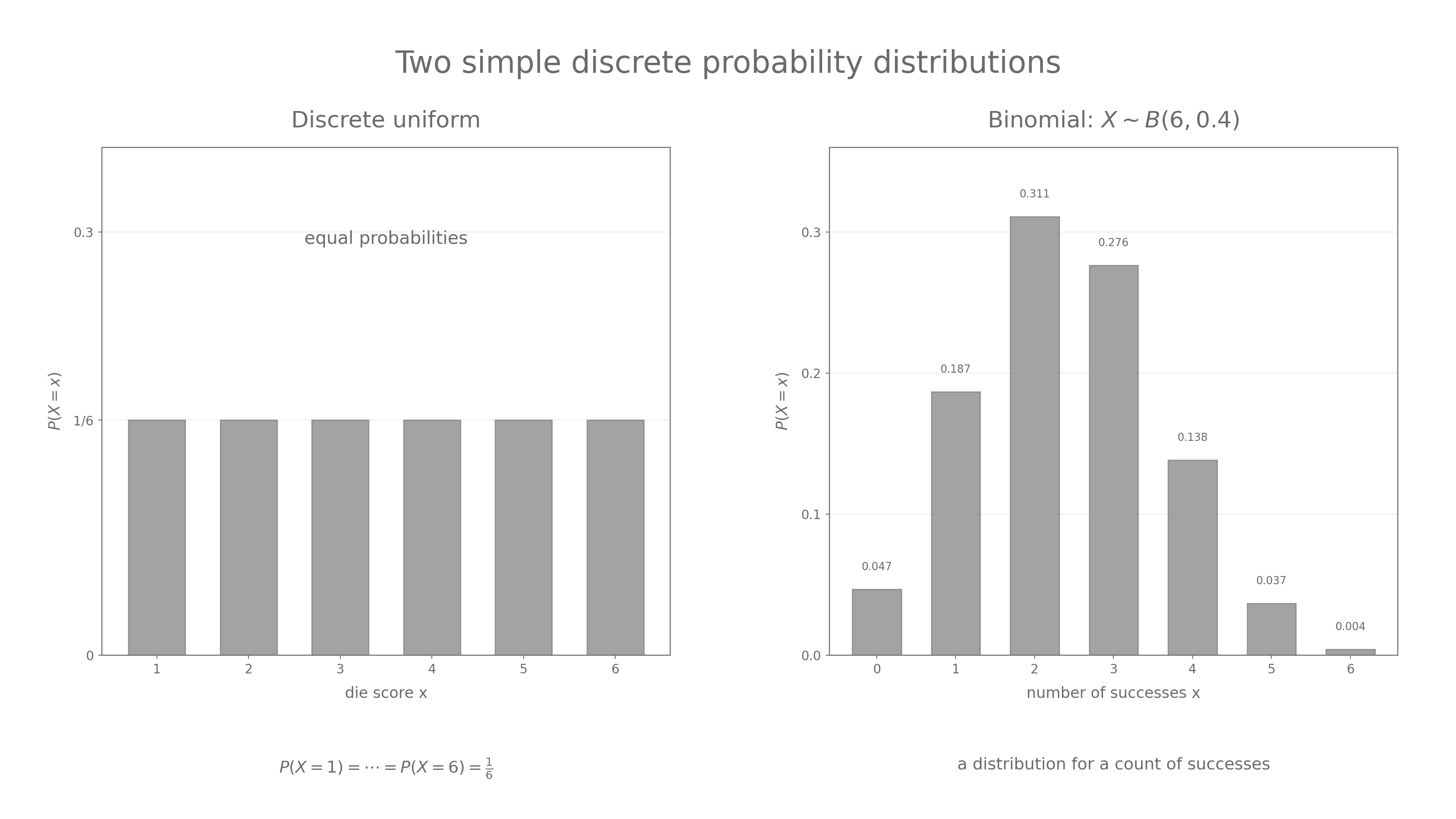
To find an event's probability, add the probabilities of the values it includes. First see this with equal sectors.

Worked example 1: equal spinner sectors

Question. A fair spinner has four equal sectors labelled $1$ , $2$ , $3$ and $4$ . Let $X$ be its score. State its distribution and find $P(X\ge3)$ .

Plan. Give each equally likely score the same probability, then add the included scores.

\begin{aligned} P(X=x)&=\frac14\quad (x=1,2,3,4) &&\text{four equal sectors}\\ P(X\ge3)&=P(X=3)+P(X=4) &&\text{list the included scores}\\ &=\frac14+\frac14=\frac12 &&\text{add disjoint outcomes} \end{aligned}

Why add? The spinner cannot land on both scores in one spin, so the outcomes are mutually exclusive.

Answer. $X$ has a discrete uniform distribution on $\{1,2,3,4\}$ , and $P(X\ge3)=\frac12$ .

Check. The full distribution sums to $4\times\frac14=1$ ; the event uses two of the four equal sectors.

Now change only the sector sizes. The labels stay the same, but equal probabilities can no longer be assumed.

Worked example 2: unequal spinner sectors

Question. A spinner has scores $1$ , $2$ , $3$ and $4$ , with $P(X=x)=kx$ . Find $k$ and $P(X\ge3)$ .

Plan. Use the total probability to find the scale factor, then add the required probabilities.

\begin{aligned} k+2k+3k+4k&=1 &&\text{all probabilities sum to one}\\ 10k&=1\quad\Rightarrow\quad k=\frac1{10} &&\text{solve for the scale}\\ P(X\ge3)&=3k+4k=\frac7{10} &&\text{include scores three and four} \end{aligned}

Why find $k$ first? The numbers $1,2,3,4$ describe relative weights; they become probabilities only after scaling their sum to $1$ .

Answer. $k=\frac1{10}$ and $P(X\ge3)=\frac7{10}$ . The distribution is discrete but not uniform.

Check. Its probabilities are $0.1,0.2,0.3,0.4$ , all nonnegative and summing to $1$ .

A familiar trap is to divide by the number of values when those values are not equally likely.

Watch out

Four possible scores do not imply $P(X=4)=\frac14$ . In the second spinner, $P(X=4)=4k=0.4$ . Equal probabilities need a reason.

Try the same scaling argument with one extra score. General discrete means and variances are outside this lesson's required calculations.

Building a binomial model

A Binomial variable counts how often one chosen outcome occurs in a fixed number of trials. If a sample contains $30$ bulbs, the random variable is the number of defective bulbs, not the condition of one bulb.

Binomial distribution

Write $X\sim B(n,p)$ when $X$ counts successes in $n$ independent trials, each with the same success probability $p$ . Each trial is classified as success or failure, and $n$ is fixed before the trials begin. The possible counts are $0,1,\ldots,n$ .

“Success” is a mathematical label: a faulty bulb can be a success if faults are what you count. A die has six faces, yet “six” versus “not six” gives two classifications. What matters is the event being counted.

Worked example 3: defining a success

Question. A very large production run has a defect probability of $0.07$ per bulb. A random sample of $30$ bulbs is inspected. Define $X$ , state a Binomial model and give the assumptions about defects.

Plan. Identify one trial, the success event and the fixed number of trials.

\begin{aligned} \text{success}&=\text{one inspected bulb is defective} &&\text{choose the counted event}\\ n&=30,\qquad p=0.07 &&\text{read the trial parameters}\\ X&\sim B(30,0.07) &&\text{count defective bulbs} \end{aligned}

Why mention the large run? Sampling a small fraction makes any change caused by removal negligible; it does not by itself rule out faults clustered by machine or time.

Answer. $X$ is the number of defective bulbs among the $30$ . Use $B(30,0.07)$ , assuming defect statuses are independent and each sampled bulb has defect probability $0.07$ .

Check. A possible value such as $X=2$ means two faulty bulbs. A value $X=31$ is impossible.

Keep the same sampling situation and change only which outcome is called a success. The complement probability must change with it.

Worked example 4: counting the opposite outcome

Question. In the same sample, $Y$ is the number of bulbs that are not defective. State a Binomial model and relate $Y$ to $X$ .

Plan. Use the non-defective probability and keep the number of trials unchanged.

\begin{aligned} P(\text{not defective})&=1-0.07=0.93 &&\text{use the complement}\\ Y&\sim B(30,0.93) &&\text{count the new successes}\\ Y&=30-X &&\text{each bulb has one classification} \end{aligned}

Why is $p$ now $0.93$ ? It belongs to the event the variable counts, rather than to the story in general.

Answer. $Y\sim B(30,0.93)$ , under the same independence and constant-probability assumptions, and $Y=30-X$ .

Check. If two bulbs are defective, $28$ are not defective; the two counts total $30$ .

When a question asks for an assumption, name it in context: “the bulbs' defect statuses are independent” or “every bulb has the same defect probability”. Saying a probability is “independent” mixes two different ideas.

Exam tip

Write the random variable and distribution, such as $X\sim B(30,0.07)$ . A list of calculator inputs does not state a statistical model.

Now change the probability, still counting the non-defective outcome.

Finding exact binomial probabilities

For eight independent trials, exactly two successes can occur in many different positions. One particular order has probability $p^2(1-p)^6$ ; there are $\binom82=28$ such orders.

Binomial probability

For $X\sim B(n,p)$ , where $n$ is a fixed nonnegative integer and $0\le p\le1$ ,

P(X=r)=\binom nr p^r(1-p)^{n-r},\qquad r=0,1,\ldots,n.

In the formula booklet.

The combination factor counts positions, not extra trials. Here is a pleasing consequence: six fair coins have $64$ equally likely head-tail strings, but exactly three heads occurs in $20$ of them. Its probability is $\frac{20}{64}=\frac5{16}$ , while six heads has probability just $\frac1{64}$ . Equally likely strings produce unequal count probabilities.

Continue this lesson.

You’re previewing NovaLearn without an account. Create a free account to read the rest.

Create free account

Last Accessed

Pure Mathematics (Papers 1 and 2)

Statistics (Paper 3, Section A)

Mechanics (Paper 3, Section B)

Statistics 4.1 - Discrete and binomial probability distributions

What a discrete distribution tells you

Building a binomial model

Finding exact binomial probabilities

Continue this lesson.

Learn faster with Nova