Pure 6.6 - Logarithmic graphs for estimating parameters | Edexcel A-Level Mathematics

Turn curved positive data into a straight line so you can estimate a model's constants. You will choose the correct logarithmic axes for power and exponential relationships, recover parameters from a gradient and intercept, and judge how far a fitted model can be trusted.

Why logarithmic graphs make parameters visible

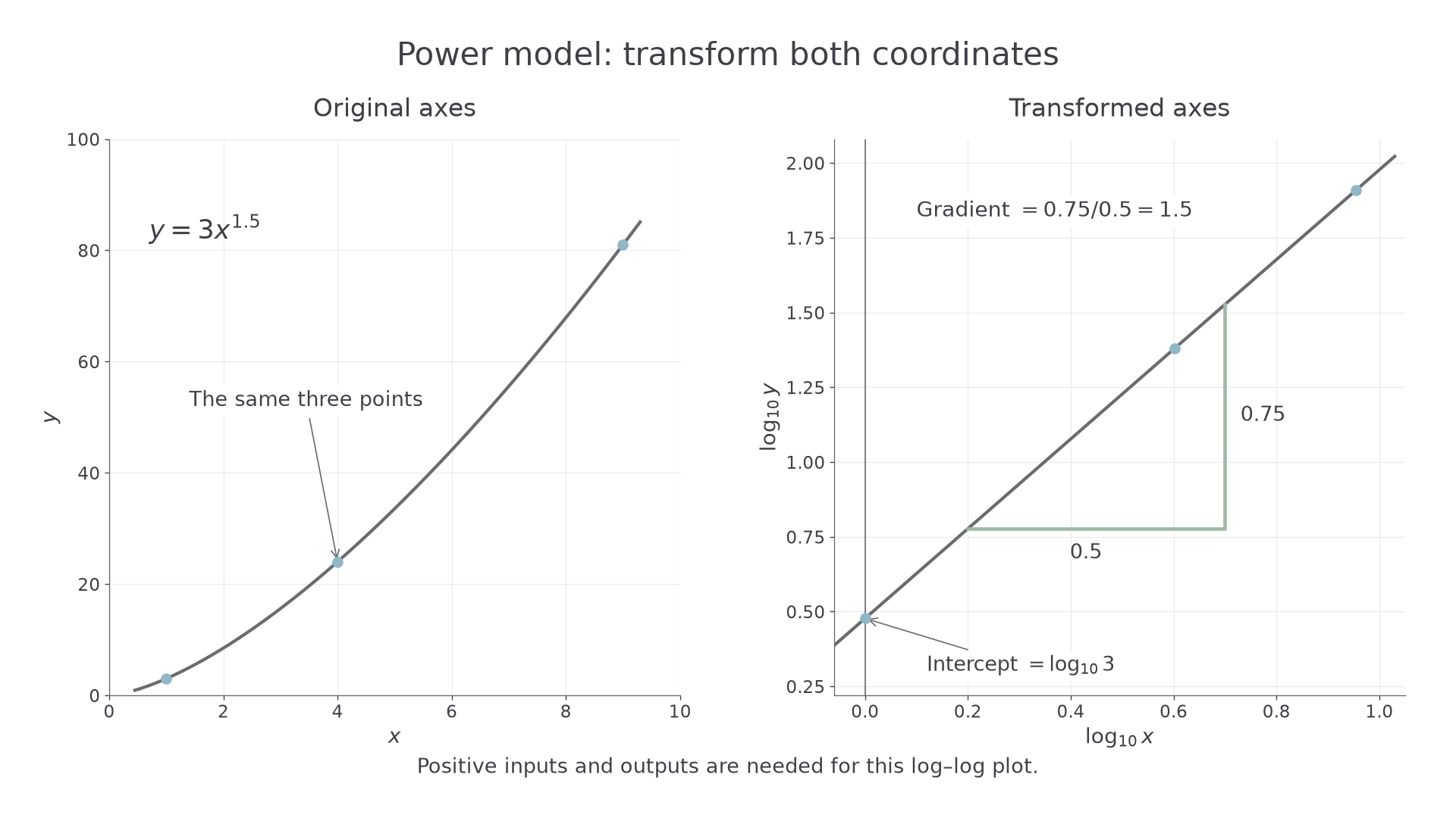
Can the curved data $(1,3)$ , $(4,24)$ , $(9,81)$ hide a straight line? They fit $y=3x^{1.5}$ . Taking base- $10$ logarithms gives coordinates approximately $(0,0.4771)$ , $(0.6021,1.3802)$ , $(0.9542,1.9085)$ , which lie on one line. The curve has become a way to read two constants with a ruler.

You already know

A straight line has form $Y=mX+c$ . For positive inputs, logarithms turn products into sums and powers into multipliers: $\log(uv)=\log u+\log v$ and $\log(u^r)=r\log u$ .

We change the variables on the axes, rather than pretending the original curve is straight. The capital letters $X,Y$ below are names for those transformed variables.

Linearisation

Linearisation transforms a relationship into the form $Y=mX+c$ . For example, plotting $\log y$ against $\log x$ makes a positive power relationship straight. Plotting the original $y$ against $x$ does not generally do so.

Here, “plot $Y$ against $X$ ” means put $Y$ vertically and $X$ horizontally. The required transformation depends on where the variable appears in the model.

Model	Vertical variable $Y$	Horizontal variable $X$	Gradient	Vertical intercept
$y=ax^n$	$\log y$	$\log x$	$n$	$\log a$
$y=kb^x$	$\log y$	$x$	$\log b$	$\log k$

Any value being logged must be positive. Thus both graphs need $y>0$ ; the power-model graph also needs $x>0$ . In an exponential-model graph, $x=0$ or a negative $x$ is allowed because we do not log $x$ . Use one logarithm base throughout; we write base $10$ explicitly for numerical graphs.

Key idea

A power model logs both variables. An exponential model logs the output but leaves the input unchanged.

The axis choice is a mathematical decision. Check it before interpreting any slope.

Estimate parameters in a power model

For $y=3x^{1.5}$ , taking logs gives $\log_{10}y=\log_{10}3+1.5\log_{10}x$ . You can see the gradient $1.5$ before calculating a single point. The same algebra works for any positive coefficient and real power on $x>0$ .

Linear form of a power model

For $y=ax^n$ , with $a>0$ and $x>0$ ,

\log y=n\log x+\log a

Plot $\log y$ against $\log x$ : gradient $n$ , intercept $\log a$ . Use the same logarithm base in both variables.

Not in the formula booklet: learn it.

The derivation uses the log laws: $\log(ax^n)=\log a+\log(x^n)=\log a+n\log x$ . These log laws are recall knowledge; the straight-line model is not supplied in the booklet.

[DIAGRAM: asset_name: A power curve becomes a straight line; asset_slug: p1_6_6_use_logarithmic_graphs_to_estimate_parameters_in_relationships_of_the_form_y_ax_n_and_y_k_b_x__diagram_01; caption: Logging both coordinates turns the power curve into a line whose gradient is the power; description: Two panels show y=3x to the power 1.5 on ordinary axes and log base 10 of y against log base 10 of x. Corresponding points are marked. The transformed intercept is log base 10 of 3, and a clear rise/run triangle shows gradient 1.5.]
Logging both coordinates turns the power curve into a line whose gradient is the power

Worked example 1: read a base-ten power model

Question. A plot of $\log_{10}y$ against $\log_{10}x$ has gradient $1.5$ and intercept $0.4771$ . Estimate the model $y=ax^n$ .

Plan. Read $n$ directly from the gradient and undo the logarithm of $a$ .

\begin{aligned} n&=1.5 &&\text{gradient is the power}\\ \log_{10}a&=0.4771 &&\text{intercept is a logarithm}\\ a&=10^{0.4771}=2.99985\ldots &&\text{take the base-ten antilog} \end{aligned}

Why this step? The intercept is $\log_{10}a$ , so writing $a=0.4771$ would leave the transformation undone.

Answer. $y\approx3.00x^{1.5}$ .

Check. At $x=1$ , $\log_{10}x=0$ and $y=a\approx3$ , consistent with the intercept. At $x=4$ , the model gives approximately $24$ .

Worked example 2 changes only the logarithm base used for the same relationship. The intercept changes, but the recovered model does not.

Worked example 2: read a natural-log power model

Question. A plot of $\ln y$ against $\ln x$ has gradient $1.5$ and intercept $1.0986$ . Estimate $a,n$ in $y=ax^n$ .

Plan. Keep the gradient as the power and use $e$ to undo a natural logarithm.

\begin{aligned} n&=1.5 &&\text{power-model gradient}\\ \ln a&=1.0986 &&\text{natural-log intercept}\\ a&=e^{1.0986}=2.99996\ldots &&\text{inverse of }\ln \end{aligned}

Why this step? An axis labelled $\ln y$ needs $e^c$ , whereas an axis labelled $\log_{10}y$ needs $10^c$ .

Answer. $a\approx3.00$ , $n=1.5$ , so $y\approx3.00x^{1.5}$ .

Check. $\ln3=1.098612\ldots$ , consistent with the rounded intercept. Both examples recover the same model.

This is a useful mathematical surprise: changing the log base stretches both axes by the same factor, so the gradient $n$ of a power-model graph stays unchanged. Negative gradients are allowed too; they describe negative powers, with $y$ decreasing as positive $x$ increases.

Watch out

Wrong: the power-model intercept gives $y$ when $x=0$ . Right: it occurs at $\log x=0$ , which means $x=1$ . The coefficient $a$ is the value there; $\log0$ is undefined.

In the next model the gradient is negative. Recover the coefficient using the stated log base exactly as before.

Estimate parameters in an exponential model

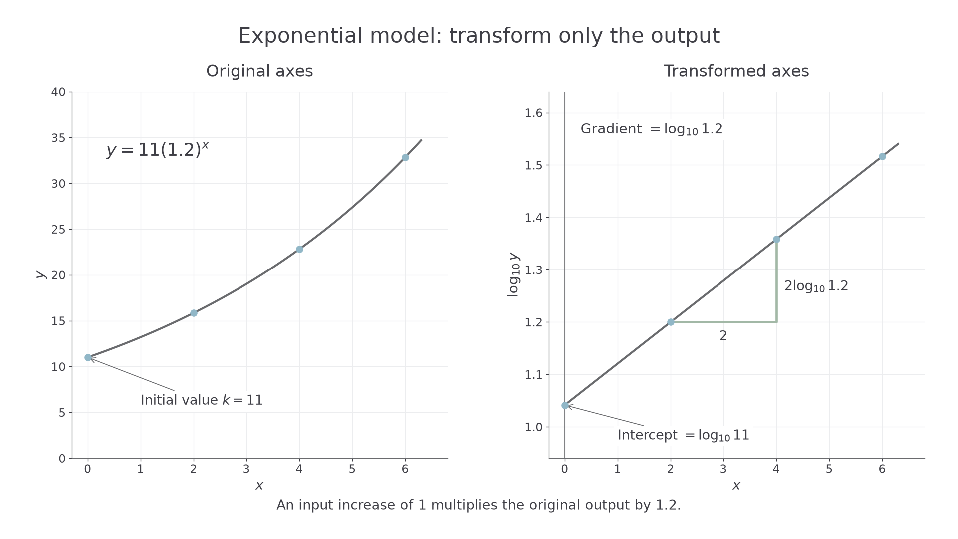
For $y=11(1.2)^x$ , each increase of $1$ in $x$ multiplies $y$ by $1.2$ . Logging the output turns that repeated multiplier into equal additions on the vertical axis.

Linear form of an exponential model

For $y=kb^x$ , with $k>0$ and $b>0$ ,

\log y=x\log b+\log k

Plot $\log y$ against $x$ : gradient $\log b$ , intercept $\log k$ . For a changing exponential model, $b\ne1$ ; $b=1$ gives a horizontal line.

Not in the formula booklet: learn it.

The derivation is $\log(kb^x)=\log k+\log(b^x)=\log k+x\log b$ . The variable $x$ is already a multiplier, so it stays untransformed.

[DIAGRAM: asset_name: An exponential curve becomes a straight line; asset_slug: p1_6_6_use_logarithmic_graphs_to_estimate_parameters_in_relationships_of_the_form_y_ax_n_and_y_k_b_x__diagram_02; caption: Logging only the output gives a straight line with gradient equal to the logarithm of the multiplier; description: Two panels show y=11 times 1.2 to the x and log base 10 of y against x. The original initial value is 11. The transformed intercept is log base 10 of 11, and a rise/run triangle identifies the gradient log base 10 of 1.2.]
Logging only the output gives a straight line with gradient equal to the logarithm of the multiplier

Worked example 3: recover both exponential constants

Question. A plot of $\log_{10}y$ against $x$ has intercept $1.0414$ and gradient $0.07918$ . Estimate $k,b$ in $y=kb^x$ , to $3$ significant figures.

Plan. Take base- $10$ antilogs of both the intercept and gradient.

\begin{aligned} k&=10^{1.0414}=11.0001\ldots &&\text{undo }\log_{10}k\\ b&=10^{0.07918}=1.199996\ldots &&\text{undo }\log_{10}b \end{aligned}

Why this step? Unlike a power-model slope, this slope is a logarithm of the parameter. Both constants need an antilog.

Answer. $k=11.0$ , $b=1.20$ , giving $y\approx11.0(1.20)^x$ .

Check. At $x=0$ , $y\approx11$ . Increasing $x$ by $1$ multiplies $y$ by approximately $1.20$ , a $20\%$ increase per input unit.

Continue this lesson.

You’re previewing NovaLearn without an account. Create a free account to read the rest.

Create free account

Last Accessed

Pure Mathematics (Papers 1 and 2)

Statistics (Paper 3, Section A)

Mechanics (Paper 3, Section B)

Pure 6.6 - Logarithmic graphs for estimating parameters

Why logarithmic graphs make parameters visible

Estimate parameters in a power model

Estimate parameters in an exponential model

Continue this lesson.

Learn faster with Nova