S2 2.2, S2 2.3, S2 2.5 - Cumulative functions and quantiles
A cumulative distribution function collects probability from left to right. Build one from a density, recover the density by differentiation, and use the two functions to locate medians, quartiles and modes.
Constructing a piecewise cumulative function
If a density rises steadily across an interval, does its midpoint divide probability in half? Not usually: the greater heights on the right give more probability to that side. Accumulated area tells you where half the probability really lies.
Cumulative distribution function
The cumulative distribution function, or c.d.f., is
The integration variable distinguishes the variable being integrated from the upper limit . The integral definition of the c.d.f. is in the formula booklet.
A c.d.f. is nondecreasing, lies between zero and one, and is continuous for a variable with a density. Below the support it is zero. Above the support it is one, even though the density there is zero. At a change of formula, carry forward the probability already accumulated.
Worked example 1: one density formula
The density is for , zero otherwise. Find for all real .
Plan. Separate values below, within and above the support.
For ,
Answer.
Check. The middle formula gives , , and increases on the support. At its midpoint, , so the midpoint does not divide probability in half.
Change the density from a single formula to two pieces. The new decision is how to preserve the area collected before the join.
Worked example 2: carrying area across a join
Find the c.d.f. for
Plan. Integrate each branch, including the first branch's area when .
For , . For ,
Answer.
Check. Both middle formulae give at the join, and the upper branch gives . Although the density jumps from one to one half, its accumulated area does not jump.
Once is known, interval probabilities are , and upper-tail probabilities are .
Watch out
For in the second example, alone forgets the probability already accumulated. A c.d.f. cannot restart at zero at an interior join.
Carry forward the first piece's area in this new distribution.
Differentiating a cumulative function
The slope of accumulated probability is density: differentiation reverses the integration that constructed .
Density from the c.d.f.
Where the derivative exists,
This relation is expected recall in S2. Differentiate each branch on its own interval, and give density zero outside the support.
At a join, a c.d.f. may have a corner. A density's value at a single endpoint can be assigned either adjoining finite value without changing probabilities; there is no need to invent a derivative where none exists. A jump in would mean a positive point probability and would not describe the continuous density model studied here.
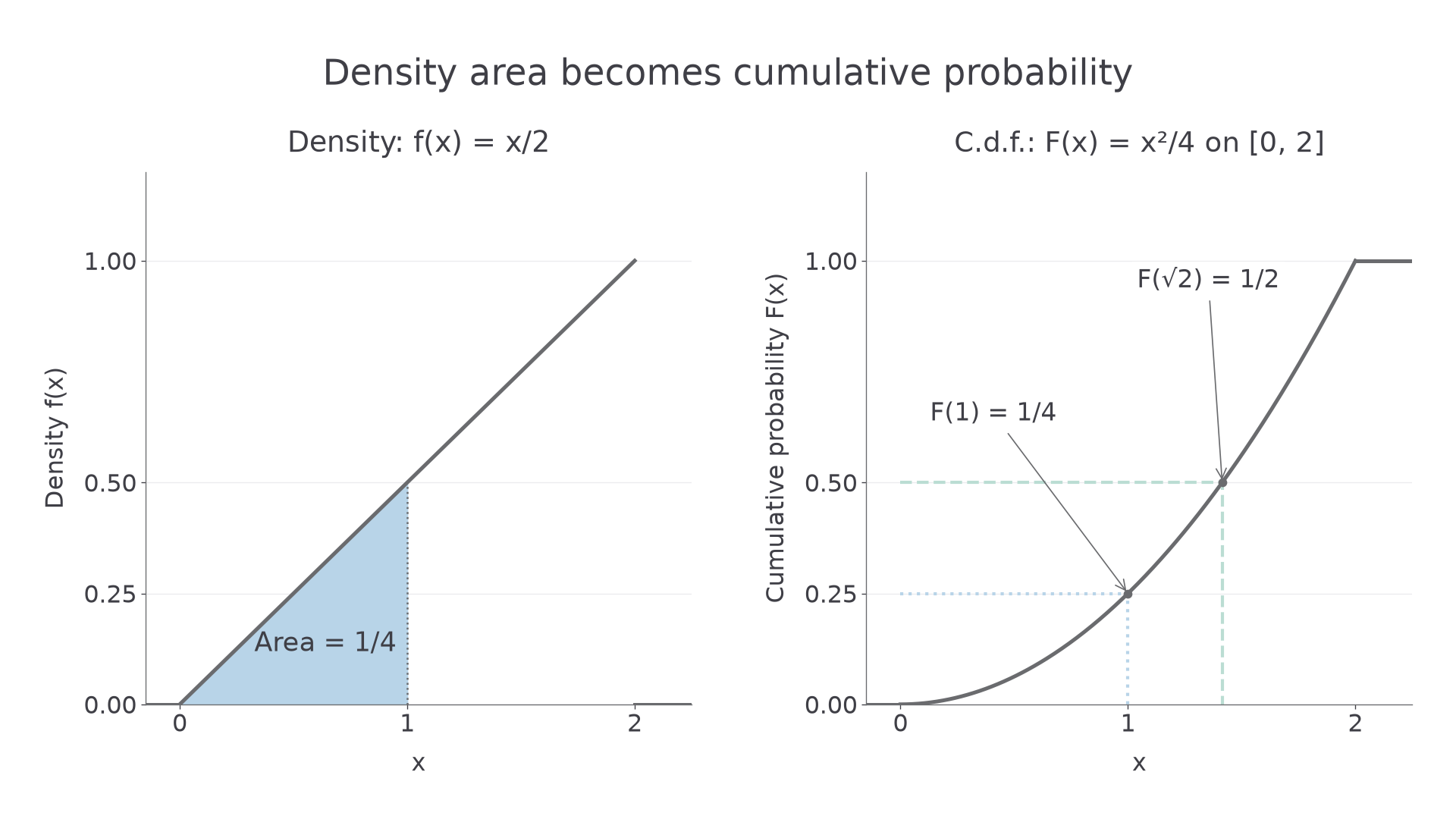
[DIAGRAM: asset_name: A density and its accumulated area; asset_slug: s2-density-cdf-link; caption: The density's area up to x becomes the c.d.f.'s height at x.; description: Side-by-side graphs of f(x)=x/2 on [0,2] and F(x)=x squared divided by 4 on [0,2], extended by constant zero and one outside the support. The left graph shades the area through x=1 as one quarter. The right graph labels F(1)=one quarter and F(square root of 2)=one half.]
Worked example 3: differentiating a power
For on , with below zero and above two, find the density.
Plan. Differentiate the polynomial branch and the constant branches separately.
Answer. on , zero otherwise.
Check. It is nonnegative, and .
Reflect the density across the midpoint of the support. The c.d.f. still increases, even though the density will now decrease.
Worked example 4: differentiating a reflected shape
For on , with the same outside branches, find the density.
Plan. Expand the cubic before applying polynomial differentiation.
Answer. on , zero otherwise.
Check. The density is nonnegative, and its integral from zero to is . Its total area is therefore one.
A cumulative function's height and slope convey different information.
Continue this lesson.
You’re previewing NovaLearn without an account. Create a free account to read the rest.
Create free account