S1 2.1 - Reading statistical diagrams
Read histograms, stem-and-leaf diagrams and box plots, including displays with unequal intervals and two groups. Use their centre and spread to make comparisons in context, and understand the information each display keeps or loses.
Histograms with unequal intervals
Can the tallest histogram bar contain fewer observations than a shorter bar? Yes: frequency depends on the bar's area, so its width matters too.
A histogram represents grouped numerical data with adjoining bars. The horizontal axis shows class boundaries. For continuous data, an interval such as includes but excludes , so adjacent classes do not overlap.
Frequency density
When the vertical axis is frequency density,
Thus bar area represents frequency. This formula is not printed in the formula booklet: learn it.
The diagram shows waiting times. Its – bar is tallest, but its narrow width means it need not have the greatest frequency.
[DIAGRAM: asset_name: Unequal histogram intervals; asset_slug: unequal-histogram-intervals; caption: The tallest bar has area 20; the wider final bar has area 30.; description: Waiting-time histogram with intervals zero to ten, ten to fifteen and fifteen to thirty minutes, frequency densities two, four and two. Each bar is labelled with its frequency twenty, twenty and thirty.]
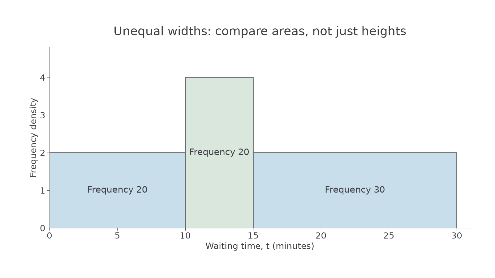
To construct the display, calculate each class width and density, use one horizontal scale and one vertical scale, then draw adjoining rectangles. If heights are measured in centimetres rather than density units, use a known bar to find the common scale. For example, density drawn as means density is drawn as .
Worked example 1: area gives a class frequency
Question. A waiting-time histogram has density on , where is measured in minutes. Find the number of observations in that class. Compare it with a bar of density on .
Plan. Multiply each density by its own class width.
Answer. The wider, shorter bar represents observations, compared with in the taller bar.
Check. The widths are in the ratio and the heights in the ratio , so the areas are in the ratio , matching .
Change only the interval requested, from a whole class to part of it. Grouped data do not reveal the individual waiting times, so we must now make an estimate.
Worked example 2: part of a bar
Question. For the same histogram, estimate the number of waiting times in .
Plan. Assume observations are spread uniformly within the – class, so the required fraction of its width gives the same fraction of its frequency.
Answer. An estimated waiting times. The word “estimated” matters because the exact positions within the class are unknown.
Check. The required interval covers two thirds of the class, so it should contain two thirds of . Equivalently, its area is .
If several classes are involved, add their whole or partial areas. A decimal estimated count may be rounded to a sensible whole number when the task asks how many people or objects.
Watch out
Do not compare frequencies by bar height when widths differ. Use areas. The modal class is the class with greatest frequency density; the class with greatest total frequency can be different.
Use the supplied intervals and densities independently of the earlier diagram.
Stem-and-leaf and back-to-back displays
A stem-and-leaf diagram retains the individual observations while arranging them in order.
The stem gives the leading digit or digits and the leaf gives the final digit. A key fixes the place value and units: is a different scale from . Repeated observations need repeated leaves, and an empty stem may be kept so that a gap in the data is visible.
A back-to-back stem-and-leaf diagram places two groups either side of shared stems. On the left, leaves increase as you move away from the stem towards the left; on the right, they increase towards the right. Read a leaf together with its stem, rather than reading the printed row as a multi-digit number. A two-sided key such as means in either group: is the central stem and each is a leaf.
[DIAGRAM: asset_name: Back-to-back response times; asset_slug: back-to-back-response-times; caption: Each leaf represents one response time; the central stem fixes the tens digit.; description: Back-to-back stem-and-leaf display. Group A has twenty-four, twenty-eight, thirty-one, thirty-one, thirty-six, forty-two and forty-seven seconds. Group B has twenty-two, twenty-five, twenty-nine, thirty-three, thirty-eight, forty-one and forty-four seconds. Stems are two, three and four. The key one bar three bar one means thirty-one seconds in either group, with three explicitly identified as the central stem.]
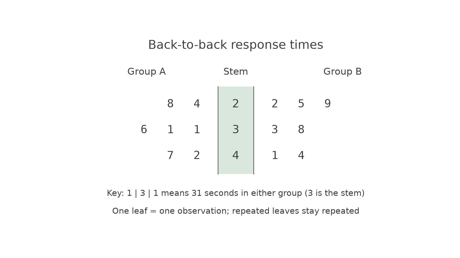
To construct one, choose stems that preserve the required precision, place each leaf beside its stem, order both sides and include a key. The shared stems allow direct comparison without hiding the raw values.
Worked example 3: reading one side
Question. Group A's back-to-back rows are , , and . The key means in either group, with the central stem. Find its median and range.
Plan. Read from the lowest stem upwards, taking the leaves nearest the stem first on the left side.
There are values, so the median is the fourth; the range uses the largest and smallest.
Answer. Median , range .
Check. Three values lie on each side of the fourth position. The two leaves on stem represent two observations, not one.
Change only the side read: the key and stems stay the same, but the right-hand leaves are read outwards towards the right.
Worked example 4: reading the other side
Question. Group B's rows are , , and , with the same key. Find its median and range and compare the medians with Group A.
Plan. Recover the seven values, then use the middle value and extremes.
Answer. Group B's median is , higher than Group A's, so its typical response time is longer by this measure. Its range is .
Check. The fourth value is , and both endpoints appear in the diagram. The median comparison concerns typical times, not every individual's time.
The diagram preserves exact values, but it can become crowded for a very large dataset.
Watch out
A leaf is one observation. Never combine leaves into , discard repeats, or assume a decimal scale without reading the key.
Read the new decimal key carefully.
Continue this lesson.
You’re previewing NovaLearn without an account. Create a free account to read the rest.
Create free account