S2 1.1, S2 1.2 - The binomial distribution

Binomial assumptions and model choice

If a player succeeds on three quarters of their attempts, should you expect exactly six successes in eight attempts? Six is a useful average, but the count can vary. A distribution describes that variation.

Imagine eight attempts, each independently successful with probability $0.75$. Record each attempt as success or failure, then let $X$ count successes. The possible values are $0,1,\ldots,8$, rather than every real number between zero and eight.

“Success” names the category counted; it need not be desirable. For example, a defect can be a success in a count of defective components. A trial may have many physical outcomes, provided each is classified into one of two categories: a die throw is either a six or not a six.

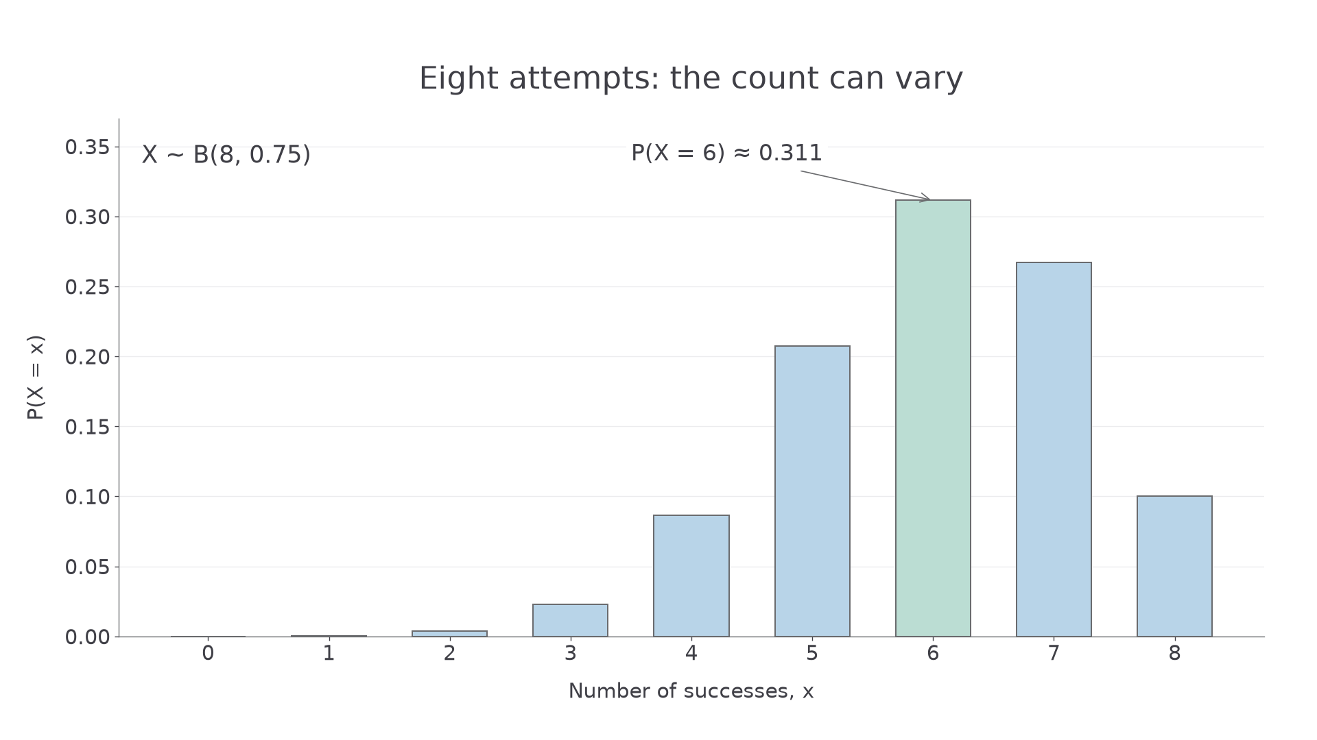
For the eight attempts, $X\sim\mathrm{B}(8,0.75)$. The picture shows that six is most likely, yet several nearby counts have substantial probability.

[DIAGRAM: asset_name: A binomial success count; asset_slug: s2-binomial-count; caption: Eight independent attempts with success probability 0.75 give a distribution of counts.; description: Bar chart of the binomial distribution with n equal to 8 and p equal to 0.75. Integer counts 0 to 8 are labelled. The bar at 6 has probability approximately 0.311 and is highlighted.]

Consider a different procedure: keep throwing a die until the first six, and count throws. The success probability is constant, but the number of trials is not fixed. This count is not binomial. Checking only one assumption is insufficient.

Apply that checklist to a new count.

Point and cumulative probabilities

A point probability selects one possible count; a cumulative probability adds all counts up to a boundary.

For three successes among ten trials, any particular ordering has probability $p^3(1-p)^7$. There are $\binom{10}{3}$ possible choices of the three successful positions, so multiply by that number. This is the same coefficient that appears in a binomial expansion.

For integer counts, “at least three” is the complement of zero, one or two. Thus $\mathrm{P}(X\ge3)=1-\mathrm{P}(X\le2)$. Likewise, “more than three” uses $1-\mathrm{P}(X\le3)$. Write the count boundaries before using your calculator or tables.

Keep the model unchanged and change just the event, from a single count to an inclusive interval.

If $p>0.5$ and you want to use the booklet tables, count failures instead: $Y=n-X\sim\mathrm{B}(n,1-p)$. For example, $X\ge8$ out of ten means $Y\le2$. The event must change with the variable. Direct calculation is also valid.

Use fresh parameters and retain both endpoints.