S2 2.1, S2 2.2 - Probability density functions
For a continuous measurement, probability belongs to an interval rather than to an individual value. Learn how density represents probability as area, check whether a proposed density is valid, and calculate probabilities across polynomial and piecewise densities.
Continuous values and zero point probabilities
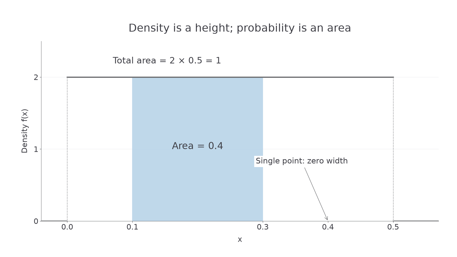
Can a density have height two when a probability can never exceed one? Yes: density is a height, while probability is an area.
A continuous random variable models measurements that can take any value in an interval, such as an unrounded length. A measuring device may display only a finite number of decimal places; that rounded display and the underlying continuous model are different things. “Exactly 1.2” on a display usually describes a small interval of true measurements.
Imagine a rectangular density of height on , and zero elsewhere. The total area is . The interval from to has probability . A single point has width zero, hence area zero.
[DIAGRAM: asset_name: Density height and probability area; asset_slug: s2-density-height-area; caption: A density may exceed one because probabilities are areas rather than heights.; description: A rectangular density of height 2 between 0 and 0.5, with the interval from 0.1 to 0.3 shaded and labelled area 0.4. A separate pointer at x equal to 0.4 is labelled single point has zero width.]
Probability density function
A probability density function, or p.d.f., , is nonnegative and has total area one. Probabilities are areas under its graph. For a variable with a density,
for any single value .
Zero probability at each point does not mean an interval has zero probability. An interval contains continuously many points; its area is found by integration rather than adding finitely many point masses. Consequently, including or excluding a finite number of endpoints does not change a continuous probability:
This differs from a binomial count, where including an endpoint can add a positive probability.
Key idea
The value is a density height. It is not .
Use the area interpretation, including its point boundary.
Normalisation and nonnegative density
A proposed density must pass two tests: it stays nonnegative and its entire area is one.
The support is the set of possible values described by the model. State where a formula applies, and give density zero outside that support. A formula such as without its interval does not define the whole distribution.
Density conditions
For a valid density,
When the density is zero outside , the integral reduces to . Use this total-area condition to find an unknown normalising constant.
Total area one alone is insufficient. For example, on integrates to one, but is negative for . It cannot be a density.
Worked example 1: an increasing density
The density is for , and zero otherwise. Find .
Plan. Set the area on the support equal to one, then check its sign.
Answer. , so on , zero otherwise.
Check. The graph is a triangle with base two and height one: its area is one. It is nonnegative throughout the support.
Reflect the shape across the midpoint of the support. Only the direction of slope changes.
Worked example 2: a decreasing density
The density is for , and zero otherwise. Find .
Plan. Integrate the new formula over the same support.
Answer. .
Check. Reflection preserves area, so the same constant is expected. Also on .
The integration variable changes; an unknown fixed constant such as does not.
Integrating for interval probabilities
Integrate a density only over the values included in the event; for a conditional probability, restrict both the numerator and the denominator appropriately.
Probability as area
For a continuous variable with density ,
The density is zero outside its support. This area formula is expected recall in S2.
If the event extends past the support, the extra area is zero. For on , an upper limit of three does not justify continuing the expression past two.
Worked example 3: an ordinary interval
For density on , zero otherwise, find .
Plan. Integrate between the two stated boundaries.
Answer. .
Check. This region under the density is a trapezium with parallel heights and , and width one. Its area is .
Continue this lesson.
You’re previewing NovaLearn without an account. Create a free account to read the rest.
Create free account