S1 2.2, S1 2.3 - Location and spread
Use measures of location in S1 2.2 to describe a typical value, and measures of dispersion in S1 2.3 to describe variability. Calculate and interpret summaries for raw and grouped data, estimate percentiles by interpolation, and recover summaries after coding.
Mean median and mode for data types
If every delivery takes ten minutes longer, its mean increases by ten minutes. Does its variability increase too? We will separate where a distribution lies from how widely its observations vary.
Discrete data take separated possible values, such as numbers of parcels. Continuous data measure quantities such as time or mass. Either can be given as individual observations, an exact-value frequency table, or a grouped table. Grouping loses the positions of observations within each class.
Measures of location
The mean is the total divided by the number of observations. The median is the central ordered value, or the average of the two central values when there are an even number. The mode is a most frequent value; there may be several modes or no useful unique mode.
The mean uses every observation and is sensitive to a few extreme values. The median depends on position and is usually less affected by extremes. A mode can describe the most common category, such as a colour, even when a numerical mean would have no meaning.
Mean from a frequency table
For values with frequencies ,
The symbol means “add all the relevant terms”. For raw data this becomes . For grouped data, substitute class midpoints for to estimate the mean. These mean formulae are not printed in the formula booklet: learn them.
Use cumulative frequencies to locate a median, rather than treating each row as one observation. For grouped continuous data, identify the median class first; interpolation in the next part will estimate a value within it. With unequal class widths, the modal class is the class with greatest frequency density, rather than necessarily greatest frequency.
Worked example 1: exact values and frequencies
Question. Values occur with frequencies , respectively. Find the mean, median and mode.
Plan. Weight each value by its frequency, then locate the middle observations in the ordered list.
Cumulative frequencies are , so the fifth and sixth values are both . The greatest frequency is , attached to .
Answer. Mean , median , mode .
Check. Relative to , the two tens contribute and the three thirties contribute , a net . Sharing this among ten values gives mean .
Change only how precisely the values are known: replace exact values by classes with the same midpoints and frequencies.
Worked example 2: grouped measurements
Question. Lengths have frequencies in the classes , , centimetres. Estimate the mean and identify the median and modal classes.
Plan. Represent each class by its midpoint, then use frequency positions and densities.
The middle observations are in . All widths are , so the greatest frequency also gives the greatest density.
Answer. Estimated mean ; both the median class and modal class are . The exact mean, median and mode are not recoverable from these grouped data.
Check. The estimate matches Example 1 because the midpoint calculation is the same. Its status has changed: the measurements need not equal their class midpoints.
The choice of summary depends on the question being asked, not on which number is quickest to calculate.
Watch out
Do not divide by the number of rows. Divide by , the total number of observations. A grouped midpoint is a representative value, not a claim that every observation equals it.
Estimate a mean from new grouped measurements.
Range interpercentile ranges and interpolation
A measure of spread says how far apart observations are; a percentile range can focus on a chosen central portion instead of the extremes.
The range is maximum minus minimum. The percentile marks the position below which approximately of observations lie. Thus , the median is , and . The interquartile range spans the middle ; spans the middle . A large range with a small IQR suggests that the extremes are much more separated than the central half.
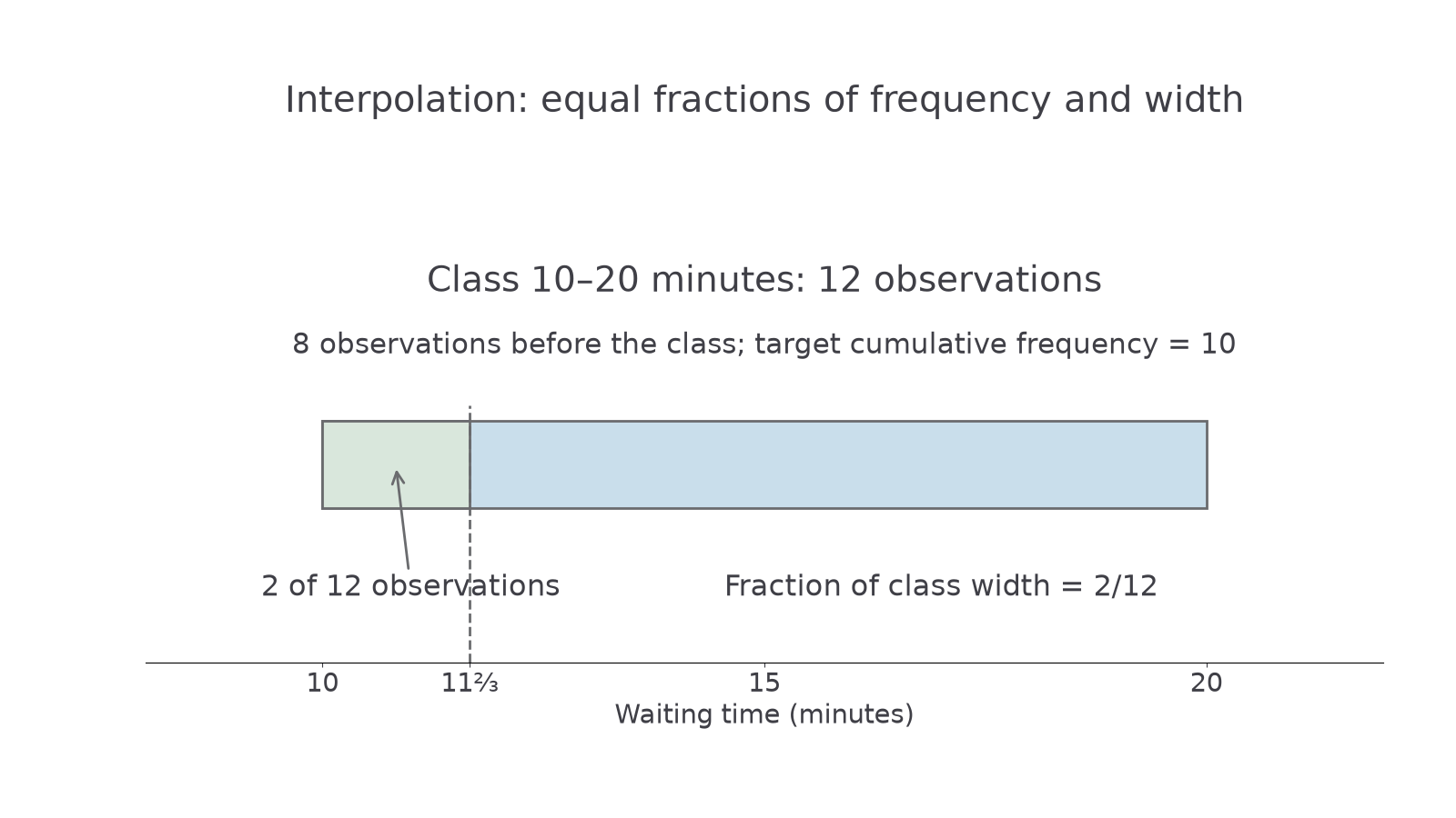
For grouped continuous data, use target cumulative frequency . If it falls within a class, linear interpolation assumes a uniform spread within that class. Covering a fraction of the class frequency therefore covers the same fraction of its width.
Grouped percentile interpolation
If the target position lies in a class with lower boundary , width , frequency and cumulative frequency before the class, then
The IQR is . These results are not printed in the formula booklet: learn them. Interpolation estimates a value; it does not recover the individual observations.
The subtraction counts how many observations into the selected class you need to go. The denominator is that class's frequency, not its cumulative frequency. If a target falls exactly at a class boundary, either adjacent-class calculation gives that boundary.
Use the following grouped waiting times:
| Waiting time , minutes | Frequency | Cumulative frequency |
|---|---|---|
| 8 | 8 | |
| 12 | 20 | |
| 20 | 40 |
[DIAGRAM: asset_name: Grouped quartile interpolation; asset_slug: grouped-quartile-interpolation; caption: Going two observations into a class of twelve means going two twelfths of the way across its width.; description: The waiting-time class ten to twenty minutes contains twelve observations, with eight observations before it. A target cumulative frequency of ten lies two of those twelve observations into the class, at eleven and two thirds minutes. The first two twelfths of the interval are shaded separately.]
Worked example 3: the lower quartile
Question. Estimate for the waiting times in the table.
Plan. Locate cumulative frequency , then interpolate in the class containing it.
The tenth position lies in , with observations before it.
Answer. Estimated lower quartile , to significant figures.
Check. Only of the class observations are needed, so the estimate is one sixth of the way from to .
Change only the requested percentile, from to . The new position lies in a different class, so its width and preceding cumulative frequency must change too.
Worked example 4: the upper quartile and IQR
Question. Estimate for the same data and hence find the IQR.
Plan. Locate cumulative frequency , interpolate, then subtract the unrounded lower quartile.
Answer. and IQR .
Check. The thirtieth position is halfway through the final class's observations, matching the midpoint of its boundaries. The IQR is positive and smaller than the full class span of minutes.
The same process gives and . Their difference, minutes, spans the estimated central . These class boundaries do not tell us the exact sample minimum or maximum, so is not necessarily the actual range.
You can also interpolate between known percentile positions. For example, moving halfway from to the median corresponds to moving halfway from cumulative proportion to , giving , provided the same uniform-spread assumption is made for that interval. This is an estimate, not information supplied by the box plot alone.
Watch out
Do not use . Quartiles refer to positions in the ordered data, not multiples of the measured values. Keep unrounded values when subtracting two estimated percentiles.
Continue this lesson.
You’re previewing NovaLearn without an account. Create a free account to read the rest.
Create free account