S1 2.4 - Skewness and outliers
Describe skewness using evidence from a distribution, apply a stated rule for outliers, and explain what an unusual observation does and does not tell you. Choose suitable measures when comparing groups whose extreme values may affect their summaries.
Reading skewness
Can a few unusually long waits change which service looks quicker? To answer fairly, first look at the direction and shape of the spread, rather than relying on one average.
Skewness
A distribution has positive skewness when its longer tail extends towards larger values, and negative skewness when its longer tail extends towards smaller values. A symmetric distribution has no directional skew. “Positive” and “negative” describe the direction of the tail, not whether the observations themselves are above or below zero.
On a histogram, look along the horizontal scale for the direction in which the tail stretches. On a box plot, compare whisker lengths and the median's position inside the box. For example, is evidence of more spread above the median within the middle half, suggesting positive skewness. Use the whole available display: quartiles alone do not establish the exact shape of the entire distribution.
[DIAGRAM: asset_name: Skewness from box-plot evidence; asset_slug: skewness-box-evidence; caption: Reflecting the distribution reverses the skew but preserves its spread.; description: Two horizontal box plots. The positively skewed example has summary zero, eight, twelve, twenty-four, forty-two. The negatively skewed reflected example has summary zero, eighteen, thirty, thirty-four, forty-two. Each of the five summary positions is labelled.]
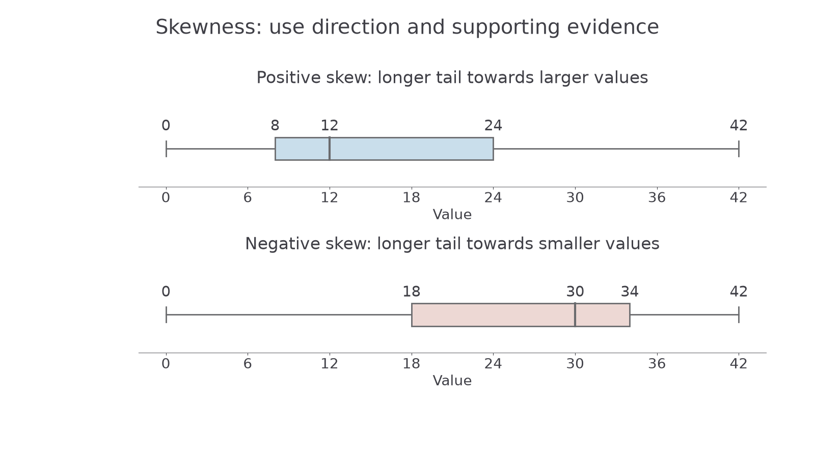
A long right tail often pulls the mean above the median; a long left tail often pulls it below. If both mean and median are supplied, that comparison can support a judgement. Do not invent a mean from a box plot: it is not one of the plotted summaries. Neither a single summary comparison nor symmetry alone determines every detail of a distribution.
Worked example 1: positive skew with reasons
Question. A box plot has minimum , , median , and maximum . Describe the skewness, giving evidence.
Plan. Compare the spread on either side of the median and check the whiskers.
The upper whisker is , compared with for the lower whisker.
Answer. The plot suggests positive skewness: both the upper half of the box and the upper whisker are longer, so the spread extends further towards larger values.
Check. The median is nearer the lower box edge, consistent with the greater spread on its upper side. No value for the mean was assumed.
Change only the direction of the scale by reflecting every value through , using . Distances stay the same but left and right swap.
Worked example 2: reversing the direction
Question. The reflected distribution has minimum , , median , and maximum . Describe its skewness with evidence.
Plan. Make the same comparisons on the new summary.
The lower whisker is , while the upper whisker is .
Answer. The plot suggests negative skewness because the spread extends further towards smaller values.
Check. Its IQR is , the same as before reflection. Reflection changes skew direction without changing distance-based spread.
Use evidence you can actually calculate or see.
Watch out
“All the values are positive, so the skew is positive” is wrong. Name the longer-tail direction and support it with the plot or a comparison of supplied summaries.
Interpret a fresh quartile pattern.
Applying a stated outlier rule
An outlier rule supplies a consistent way to flag observations that are unusually far from the main body of the data.
Outlier
An outlier is an observation judged unusually far from the others under the criterion being used. Different rules can flag different observations; apply the rule stated in the question.
One possible rule flags values below or above . Those two thresholds are called fences. This rule is an example, not a rule to impose on every question. Another question may use a different multiplier or a criterion based on the mean and standard deviation. For example, if the stated rule is “more than two standard deviations above the mean”, with mean and standard deviation , its upper threshold is . A value of is flagged, whereas is not. The rule alone supplies the criterion; no assumption about a particular distribution shape is needed for this classification.
If the wording says “below” or “above”, equality with a fence does not count as an outlier. For a box plot with separate outliers, draw each outlier as an individual point or cross on the same scale. Extend whiskers to the smallest and largest observed values that are not outliers, rather than automatically to the fences.
[DIAGRAM: asset_name: Outlier fences and observed whisker endpoints; asset_slug: outlier-fences-and-whiskers; caption: The outlier is plotted separately; the whiskers stop at actual non-outlying observations.; description: A box plot with lower quartile ten, median fourteen and upper quartile eighteen, non-outlying endpoints four and twenty-five, and an outlier at thirty-five. The stated one-point-five-IQR fences are minus two and thirty, drawn as dashed reference lines rather than whisker endpoints.]
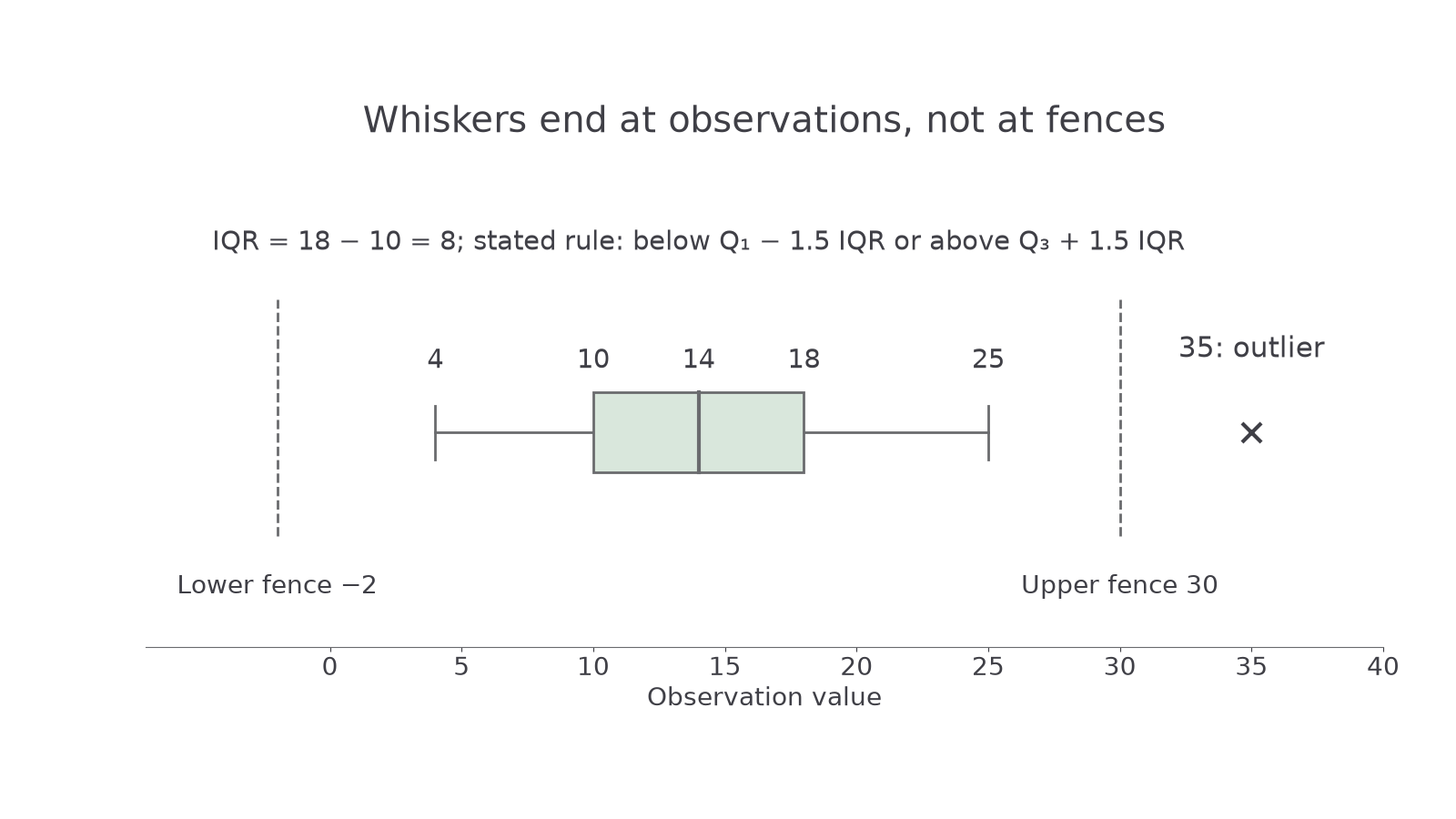
Worked example 3: applying the supplied fences
Question. A dataset has , , minimum , maximum , and next-largest observation . Using the rule “below or above ”, identify outliers and state the box-plot whisker endpoints.
Plan. Calculate the IQR and both fences, then compare the extreme observations with them.
Answer. Only is an outlier. Plot it separately. The whiskers end at observed values and , not at and .
Check. Every remaining observation lies between and , which are both inside the fences. The largest observation satisfies .
Change only the rule's multiplier from to , leaving the data unchanged.
Continue this lesson.
You’re previewing NovaLearn without an account. Create a free account to read the rest.
Create free account