S2 1.1–S2 1.3 - The Poisson distribution
Use the Poisson distribution to count events over time or space. Learn how its parameter changes with the interval, calculate cumulative probabilities, and recognise when it gives a useful approximation to a binomial count.
Poisson assumptions and event counts
If messages arrive at an average of two per minute, can you predict the chance of receiving none in the next minute? There is no fixed number of “message trials”, so a binomial model is not the natural starting point.
A Poisson model counts events in a specified interval of time or region of space. Assume events occur independently, at a constant average rate, with a negligible chance of two or more events in a sufficiently short interval. For messages, this means one arrival does not trigger another, the average rate is stable over the period, and arrivals do not come in inseparable batches. “Random” alone does not state these assumptions.
Poisson distribution
Write , where is the expected number of events in the specified interval. The possible counts are , with no finite upper bound.
A model for messages arriving in one minute can differ from a model for messages arriving in an hour. The parameter is an expected count for the chosen interval, not a rate without units attached.
Poisson point probability
For ,
In the formula booklet. Remember .
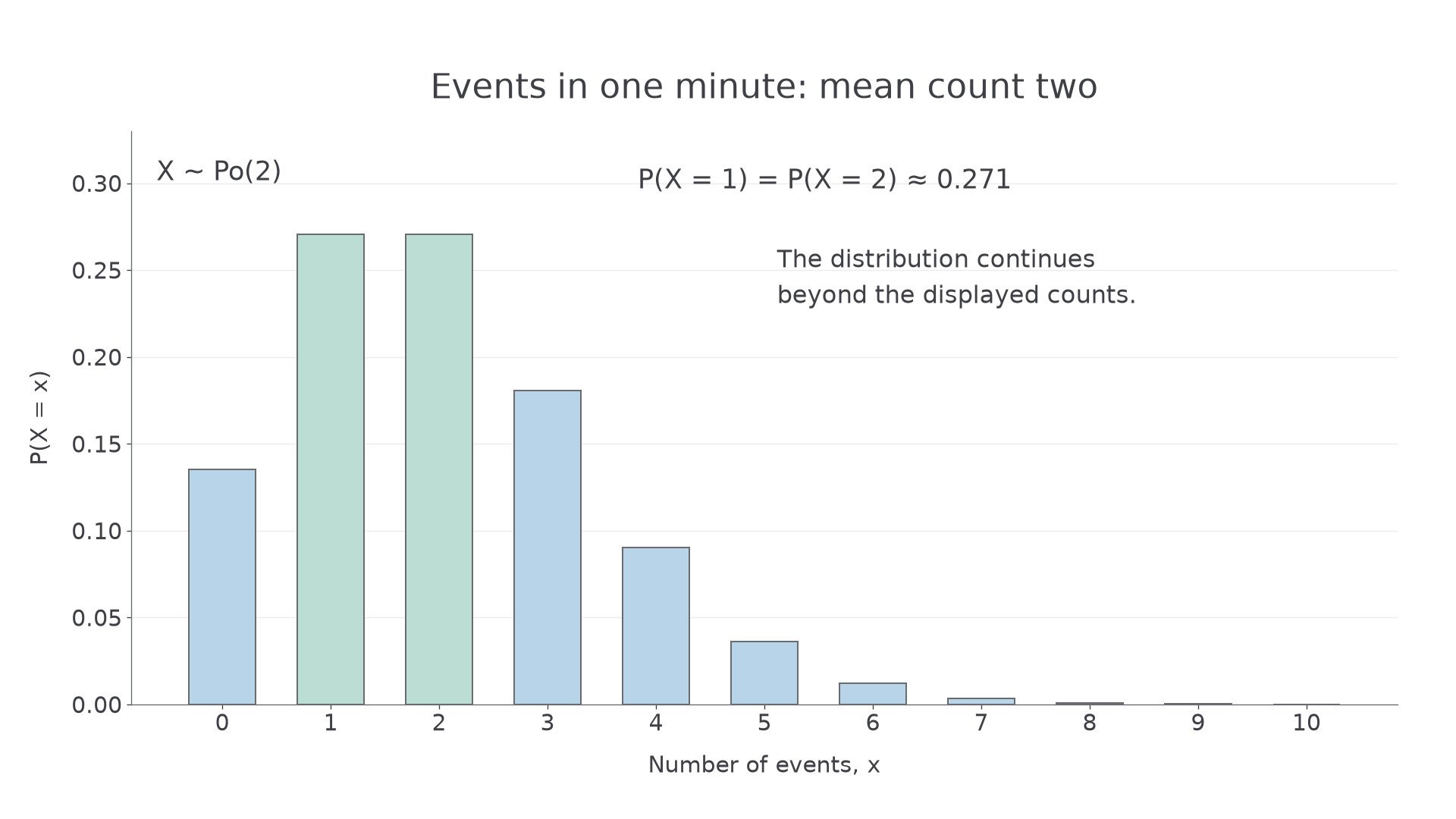
For mean two, counts near two are common, but zero and larger counts remain possible.
[DIAGRAM: asset_name: A Poisson event count; asset_slug: s2-poisson-count; caption: A Poisson mean of two gives positive probabilities at every nonnegative integer count.; description: Bar chart of the Poisson distribution with lambda equal to 2, displaying counts 0 through 10. The bars at 1 and 2 are equal and tallest. A note states that the distribution continues beyond the displayed counts.]
Worked example 1: a probability from the mean
Messages follow a Poisson model with mean two per minute. Find the probability of three messages in a minute.
Plan. Use the point formula with and .
Answer. , to three significant figures.
Check. The booklet cumulative values give , agreeing at table precision.
Change which information is unknown: two adjacent count probabilities can determine the mean. Dividing cancels the common exponential factor.
Worked example 2: the mean from probabilities
For , . Find .
Plan. Divide the point formula for count three by the one for count two.
Answer. .
Check. At mean two, and ; their ratio is , as required.
The same cancellation works for any adjacent counts. Write the two probability expressions so the factorial and power cancellation is visible.
Changing the time or space interval
Doubling an interval doubles the expected count, provided the same rate applies throughout.
If events occur at mean rate per hour, the count in hours has mean . Rates per unit length or area work the same way under a constant spatial rate. Keep the units consistent: fifteen minutes is of an hour, not hours.
Adding Poisson counts
Independent Poisson counts add:
For a constant-rate process, disjoint interval counts are independent, so the mean scales with interval length. This addition rule is not printed as a separate formula in the booklet.
Do not add two overlapping interval counts as though they were independent: events in their overlap would be counted twice.
Worked example 3: a shorter interval
Calls follow a Poisson model at mean rate 12 per hour. Find the probability of no calls in 15 minutes.
Plan. First convert the rate into a mean for fifteen minutes.
Answer. .
Check. Four disjoint fifteen-minute intervals together have mean , matching the hourly model.
Change only the observation length to thirty minutes. The expected count doubles, while the event remains “no calls”.
Worked example 4: a longer interval
For the same call process, find the probability of no calls in 30 minutes.
Plan. Use the mean for half an hour, not the hourly rate.
Answer. .
Check. No calls in both independent fifteen-minute halves has probability . A longer interval makes zero calls less likely.
The same scaling applies to, for example, defects per metre of a long cable if a constant-rate independent-event model is credible.
Continue this lesson.
You’re previewing NovaLearn without an account. Create a free account to read the rest.
Create free account