D1 3.2–D1 3.4 - Travelling salesman bounds

Practical and classical tours and the triangle inequality

How could you prove that a delivery tour is shortest without listing every possible order of visits? Find a feasible tour giving an upper limit, and a calculation showing that no tour can be shorter than a lower limit.

This problem visits vertices. Route inspection instead covers every edge. The two demands can produce very different journeys.

The repeated start at the end is the necessary exception to “exactly once”. The classical networks here are complete, undirected and satisfy the triangle inequality: travelling directly is no longer than travelling through another vertex. For example, lengths $AB=3,BC=4,AC=7$ satisfy $AC\le AB+BC$. If a road $AC$ itself has length $10$, the road weights do not satisfy that inequality, since $10>3+4$. Using shortest journey distances instead replaces that entry by $7$.

A bound is not a claim that the optimum equals it. If a lower bound and a feasible tour have the same length, however, their equality proves the optimum.

Identify the exact classical demand.

Complete shortest-distance networks

A practical road network may lack direct roads between some towns; a complete shortest-distance network records the shortest journey between every pair.

Use the pictured undirected road network: $AB=2,BC=4,CD=4,DA=4,BE=4,CE=4,DE=8$, all in kilometres. A missing direct edge does not mean the towns cannot be reached.

[DIAGRAM: asset_name: Roads and shortest journey distances; asset_slug: salesman-road-network; caption: The missing road AE becomes a shortest-distance connection of 6 km, via B.; description: A weighted undirected road network with edges AB 2 BC 4 CD 4 DA 4 BE 4 CE 4 DE 8. A blue highlighted two-edge journey follows A B E of total length 6, without adding an extra road.]

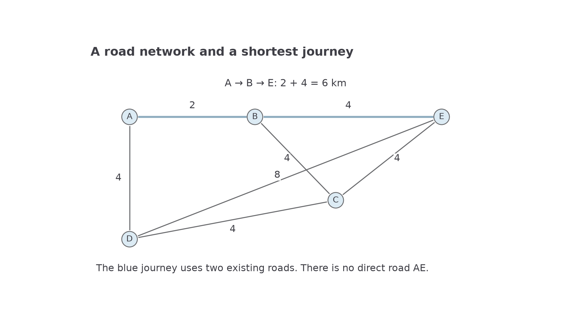
For each pair, inspect possible routes or apply Dijkstra's algorithm. Put the shortest total in the corresponding table entry. This is a distance table, not the direct-edge adjacency matrix used earlier. It is symmetric here because roads are undirected. The triangle inequality holds automatically: a journey via a third town is one available option, so the shortest journey cannot be longer than it.

Change only road $DE$, reducing it from $8$ to $3$. A changed road can improve several pair distances, so check all affected routes.

A tour edge in the completed network may expand into several roads in reality. Expanding every edge of a classical tour produces a practical tour in the road network, possibly revisiting intermediate towns. Conversely, shortcutting repeated vertices in the complete distance network cannot increase length. This connects the two models.

Nearest-neighbour upper bounds

Nearest neighbour builds an actual tour by making a local choice from the most recently visited vertex.

Start at the specified vertex. Go to the nearest unvisited vertex; repeat from your new position until every vertex has been visited. Then return to the start and add that final distance. Unlike Prim's algorithm, do not search from all included vertices. Ties permit either nearest choice unless the question supplies a rule.

Use the original complete table from Example 1. For the examples below break a tie by alphabetical order, so that the trace can be followed exactly.