D1 5.2, D1 5.3 - Solving linear programs
Draw the feasible region of a two-variable linear program, then optimise using vertices or a sliding objective line in D1 5.2. In D1 5.3, restrict the answer to feasible integer points when the context requires whole objects, and interpret the optimal plan with its units and unused resources.
Feasible regions
What if the most profitable point on a graph calls for drums of one product and of another? The graph can solve a continuous model exactly, but a whole-drum requirement changes which points we may choose. First we need to know which plans satisfy the restrictions at all.
The feasible region consists of points satisfying every constraint together. Draw each boundary as an equality, then test which side satisfies its inequality. For , the point gives , so choose the side containing the origin. If the test point lies on a boundary, choose a different point: equality cannot distinguish the two sides.
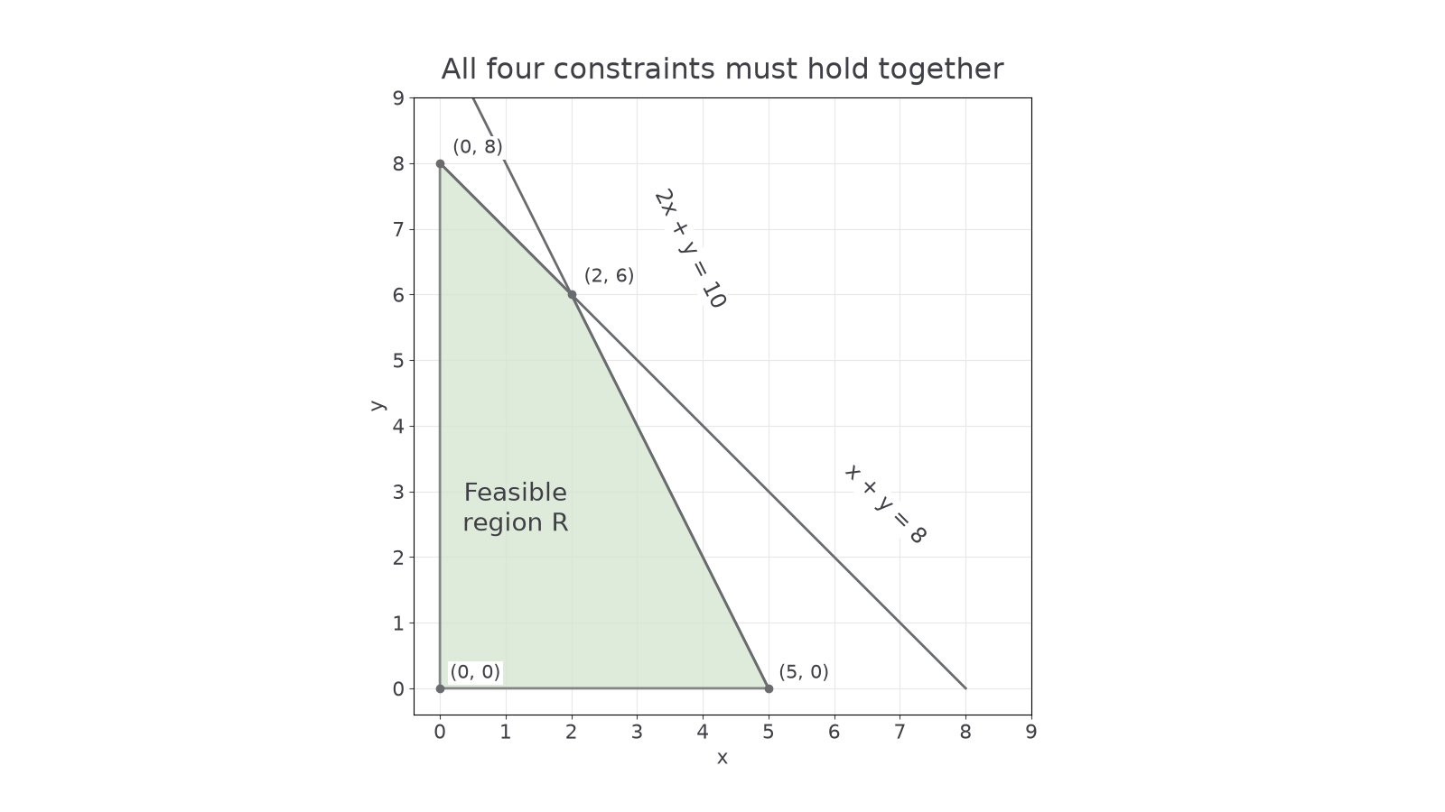
Nonnegativity restricts us to the first quadrant, including its axes. Non-strict inequalities include the boundary lines; draw them solid. State your shading convention clearly. The diagram below colours the feasible region green; an exam diagram may instead shade excluded regions and leave the feasible region unshaded.
[DIAGRAM: asset_name: A two-variable feasible polygon; asset_slug: linear-feasible-region; caption: The green polygon includes its boundaries and satisfies every inequality.; description: First-quadrant feasible polygon for x+y at most8 and2x+y at most10, with vertices(0,0),(5,0),(2,6),(0,8), both sloping boundaries labelled and solid.]
Worked example 1: finding the feasible polygon
Find the vertices of the region satisfying
Plan. Draw the boundary lines, identify the common permitted region, and solve where its edges meet.
The sloping boundaries have intercepts and . Their intersection satisfies
On the -axis the tighter limit is ; on the -axis it is .
Answer. Vertices , joined by the included boundaries shown.
Check. Each vertex satisfies all four inequalities. The tempting intercept fails , so it is not a feasible vertex.
Change only the second resource limit from to . The permitted side remains the same, but the vertices move.
Worked example 2: a changed capacity
Find the vertices when the constraints are
Plan. Recalculate the changed axis intercept and the two-line intersection.
The -axis bound is now , while remains the tighter -axis bound.
Answer. Vertices .
Check. At , and . The original region is contained in this enlarged region, as expected when a capacity increases.
Watch out
A boundary intersection is a candidate vertex, not automatically a feasible one. Check every constraint, including the axes. Contradictory restrictions can give an empty feasible region; a region extending indefinitely is unbounded.
Use the equations, rather than a graph reading alone, when exact coordinates are needed.
Vertex and objective-line methods
A linear objective changes at a constant rate, so a straight-edged feasible region allows two equivalent optimisation methods.
For a nonempty bounded polygon, a maximum and minimum occur at vertices. Evaluate the objective at all its vertices and compare. If the objective is constant along an edge at the optimal value, every point on that edge is also optimal; the optimum need not be unique.
The ruler method, or objective-line method, uses the family
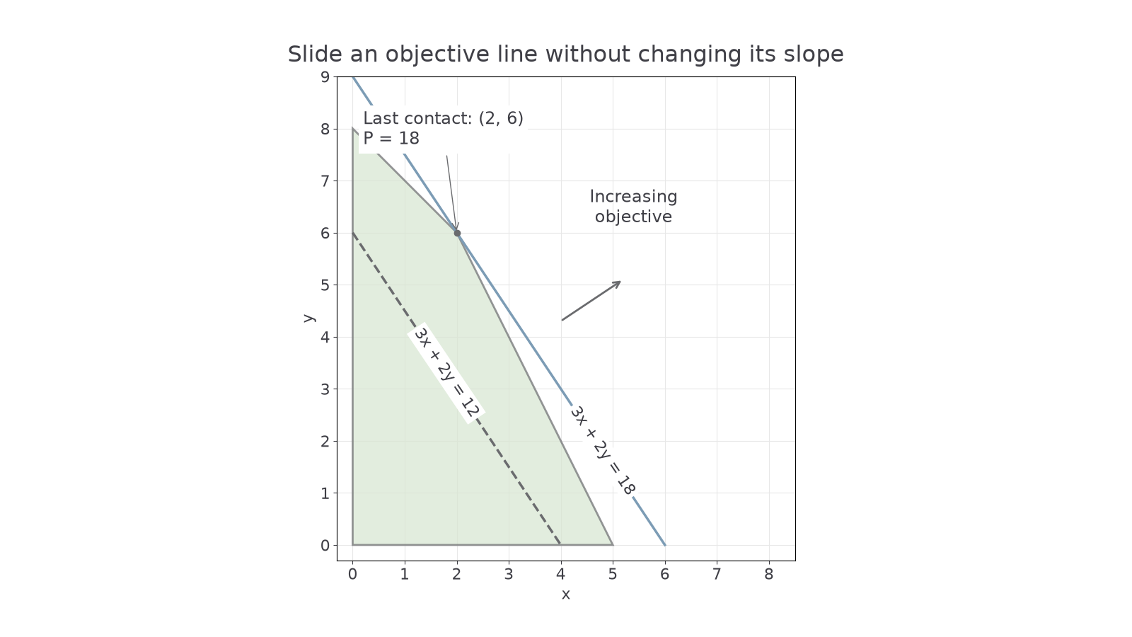
For fixed , these lines are parallel as changes. Draw a convenient line, then slide a ruler parallel to it in the direction of increasing for a maximum, or decreasing for a minimum. The last feasible contact gives the optimum. Check the direction with a test point: moving away from the origin is not a universal rule when objective coefficients have different signs. With , the gradient is ; a zero coefficient may give horizontal or vertical lines instead.
[DIAGRAM: asset_name: Parallel profit lines; asset_slug: linear-objective-lines; caption: Parallel objective lines increase until their last feasible contact at (2, 6).; description: The original polygon with vertices(0,0),(5,0),(2,6),(0,8), dashed line3x+2y=12 and parallel line3x+2y=18 touching(2,6). An arrow to the upper right indicates increasing objective.]
Worked example 3: a unique maximum
Maximise subject to
Plan. Compare the four vertex values; use a sliding line to check which corner is last touched.
| Vertex | |
|---|---|
| 0 | |
| 15 | |
| 18 | |
| 16 |
Answer. Maximum at .
Check. Lines have gradient . Sliding from towards larger values reaches the last contact at , where . No feasible vertex has a larger value. For a minimum, the same table gives at .
Change only the objective to . It is now parallel to one of the feasible edges.
Worked example 4: an entire optimal edge
Maximise over the same feasible region.
Plan. Compare vertices and inspect the edge between tied optimal vertices.
The segment from to lies on .
Answer. Maximum , attained at every point on that whole segment, including its endpoints.
Check. The constraint already says ; every feasible point on the segment achieves equality. The ruler touches an edge instead of a single corner.
A graph locates the optimal corner or edge; simultaneous equations give exact coordinates where required. If a region is unbounded, check whether the objective can improve without limit before claiming a finite optimum.
Integer feasible points
When variables count whole objects, only lattice points with integer coordinates are allowed, even if a fractional point is the continuous optimum.
Consider
and maximise . The sloping boundaries intersect at
where . Rounding both coordinates gives , which breaks both constraints. Rounding both down gives a feasible point , but its value is not best. Neither rounding rule solves an integer optimisation problem.
Continue this lesson.
You’re previewing NovaLearn without an account. Create a free account to read the rest.
Create free account