P2 5.1 - Exponential functions | Edexcel A-Level International Mathematics

Understand how a variable exponent produces growth or decay, and use exact values to describe exponential graphs. You will identify their intercepts and asymptotes, including after a vertical translation.

Positive bases and exponential growth

If a quantity doubles at each step, can its graph ever pass through zero? Starting with one gives the values $1,2,4,8$ , but extending the rule backwards gives $1/2,1/4,1/8$ . The values become small without becoming zero. We will explain the complete graph, including what happens between whole-number steps.

You already know that $2^{-1}=1/2$ and $2^{1/2}=\sqrt2$ . An exponential function lets the exponent itself vary: $y=2^x$ . It differs from $y=x^2$ , where the base varies and the exponent stays fixed.

Exponential function

An exponential function has the form $y=a^x$ , where the constant base satisfies $a>0$ and $a\ne1$ . Its domain is all real $x$ , and its values are positive.

A positive base makes the function real-valued throughout this domain. For instance, $(-2)^{1/2}$ is not real, so a negative base cannot give this all-real-domain exponential graph. Base $1$ is excluded because $1^x=1$ is constant.

For $a>1$ , increasing $x$ increases $a^x$ . In particular,

a^{x+1}=a\,a^x.

Every increase of one in $x$ multiplies the output by the same factor $a$ ; it does not add the same amount. This is exponential growth. More generally, an increase of $h>0$ multiplies the output by $a^h>1$ .

Worked example 1: evaluating a growth function

Question. For $y=3^x$ , find $y$ when $x=-2,0,1/2,2$ .

Plan. Read a negative index as a reciprocal, zero as one and a half as a square root.

\begin{aligned} 3^{-2}&=\frac1{3^2}=\frac19\\ 3^0&=1\\ 3^{1/2}&=\sqrt3\\ 3^2&=9 \end{aligned}

Answer. The outputs, in the requested order, are $1/9,1,\sqrt3,9$ .

Check. At the intermediate input $x=1$ , the output is $3$ . Each whole step from $x=0$ to $1$ to $2$ multiplies by $3$ , giving $1,3,9$ .

Change only the base from $3$ to $9$ . The same index meanings apply, but the growth over each unit interval is larger.

Worked example 2: changing the growth factor

Question. For $y=9^x$ , find $y$ when $x=-2,0,1/2,2$ .

Plan. Use the same four index rules with the new base.

9^{-2}=\frac1{81},\qquad9^0=1,\qquad 9^{1/2}=3,\qquad9^2=81.

Answer. $1/81,1,3,81$ .

Check. Since $9^x=(3^x)^2$ , squaring the four answers in Example 1 gives exactly these four outputs.

The common starting value is not a coincidence: every allowed base has $a^0=1$ .

Watch out

$3^{x+1}=3\times3^x$ , not $3^x+1$ . Equal steps in the input give equal multiplication factors in the output.

Try a different base with the same index meanings.

Decay with a base between zero and one

Multiplication can make a positive number smaller: multiplying repeatedly by $1/2$ halves it at every step.

For $y=(1/2)^x=2^{-x}$ , the outputs at $x=0,1,2$ are $1,1/2,1/4$ . Moving right makes the graph fall; moving left makes it rise. These are the values of $2^x$ with the sign of the input reversed, so the two graphs are reflections in the $y$ -axis.

Exponential decay

For $0<a<1$ , $y=a^x$ is an exponential decay function. It is decreasing: a larger input has a smaller output. Each increase of one in $x$ multiplies the output by $a$ , and every output remains positive.

For any positive input step $h$ , the multiplying factor $a^h$ lies between zero and one. The decrease is therefore continuous, rather than confined to the integer points.

Worked example 3: a decay table

Question. Find the outputs of $y=(1/2)^x$ at $x=-2,-1,0,1,2$ .

Plan. Use reciprocals at negative inputs, then halve the output at each step to the right.

\left(\frac12\right)^{-2}=4,\quad \left(\frac12\right)^{-1}=2,\quad \left(\frac12\right)^0=1,\quad \left(\frac12\right)^1=\frac12,\quad \left(\frac12\right)^2=\frac14.

Answer. $4,2,1,1/2,1/4$ .

Check. Consecutive outputs have ratio $1/2$ : for example, $(1/4)/(1/2)=1/2$ . The negative-input values are greater than one, as the reciprocal rule predicts.

Change only the base to $1/4$ . Each whole step now quarters the output.

Worked example 4: a smaller decay base

Question. Find the outputs of $y=(1/4)^x$ at $x=-2,-1,0,1,2$ .

Plan. Start from $y=1$ at $x=0$ , dividing by $4$ to move right and multiplying by $4$ to move left.

\begin{array}{c|ccccc} x&-2&-1&0&1&2\\\hline y&16&4&1&1/4&1/16 \end{array}

Answer. $16,4,1,1/4,1/16$ .

Check. $(1/4)^x=((1/2)^x)^2$ ; squaring Example 3's outputs reproduces the entire table.

A negative exponent reverses the fraction; it does not make the output negative.

Watch out

$(1/4)^{-2}=16$ , not $-1/16$ . A decay function falls as $x$ increases, but it still has positive values at every real input.

Use the same table method with a new decay factor.

Graphs intercepts and asymptotes

An exponential graph passes through $(0,1)$ and approaches the horizontal axis at one end without meeting it.

For growth, the values get arbitrarily small as $x$ becomes more negative. For decay, they get arbitrarily small as $x$ becomes more positive. At every finite input, however, $a^x>0$ .

Horizontal asymptote

A horizontal asymptote is a horizontal line approached by a graph as the input becomes indefinitely large in one direction. Both growth and decay graphs $y=a^x$ have asymptote $y=0$ , $y$ -intercept $(0,1)$ , no $x$ -intercept and range $y>0$ .

The curve is smooth through its points. Do not join a value table with straight segments or let a sketch touch the asymptote. After a vertical translation, the asymptote moves with the curve.

[DIAGRAM: asset_name: Growth decay and a translated asymptote; asset_slug: exponential-graphs; caption: Growth and decay share an intercept and asymptote; shifting a graph down moves both.; description: Two panels. The first shows y equals two to the x and y equals one half to the x on labelled axes, meeting at zero comma one and approaching y equals zero at opposite ends. The second compares y equals two to the x with y equals two to the x minus three, marking the intercept zero comma negative two and the new dashed asymptote y equals negative three.]
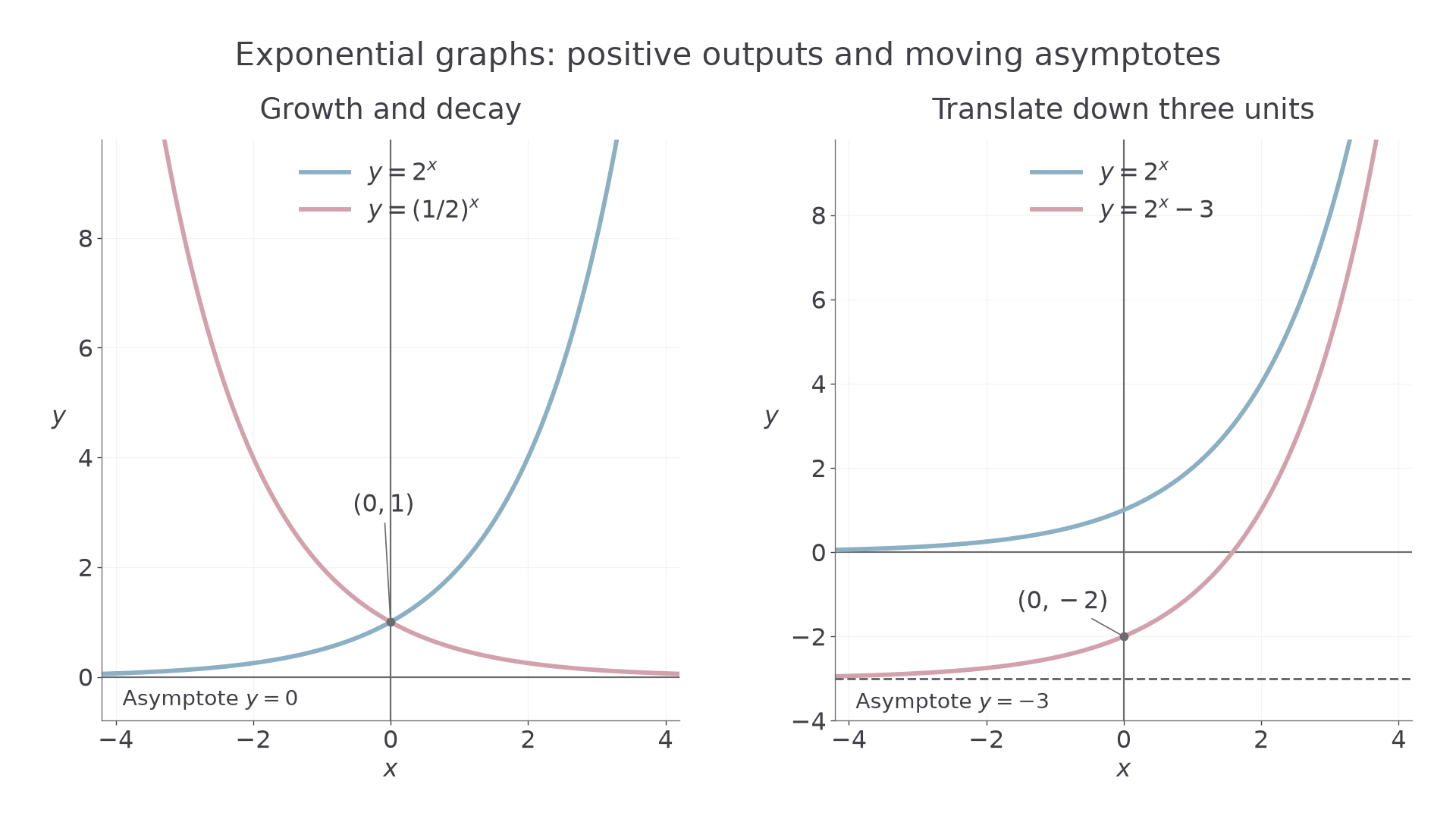
Growth and decay share an intercept and asymptote

Worked example 5: describing the basic graph

Question. Describe the intercepts, horizontal asymptote, domain and range of $y=2^x$ .

Plan. Substitute $x=0$ for the vertical intercept, then use positivity and the negative-input behaviour.

y(0)=2^0=1,\qquad 2^x>0\quad\text{for all real }x.

As $x$ decreases indefinitely, $2^x$ approaches zero. As $x$ increases, the output grows without bound.

Answer. The $y$ -intercept is $(0,1)$ ; there is no $x$ -intercept. The asymptote is $y=0$ , the domain is all real $x$ , and the range is $y>0$ .

Check. $2^{-10}=1/1024>0$ and $2^{10}=1024$ : the left tail is close to, and above, zero, while the right tail rises.

Change only the vertical position by subtracting $3$ . The domain and increasing shape stay the same, while every output decreases by $3$ .

Worked example 6: translating the graph

Question. Describe the intercepts, horizontal asymptote, domain and range of $y=2^x-3$ . Give an equation determining its $x$ -intercept.

Plan. Shift the previous graph down three units, and set each coordinate to zero in turn.

y(0)=1-3=-2,\qquad y=0\ \Longleftrightarrow\ 2^x=3.

The equation $2^x=3$ has one solution between $1$ and $2$ , since $2^1<3<2^2$ and the function increases. A later lesson will calculate it.

Answer. The $y$ -intercept is $(0,-2)$ . There is one $x$ -intercept, where $2^x=3$ . The asymptote is $y=-3$ , the domain is all real $x$ , and the range is $y>-3$ .

Check. At $x=-10$ , $y=-3+1/1024$ , just above the new asymptote. At $x=1$ and $2$ , the outputs are $-1$ and $1$ , confirming a crossing between them.

The opening doubling function never reaches zero because all its powers are positive. A translated version can cross an axis: the restriction belongs to the original output $2^x$ , not every expression containing it.

Watch out

The asymptote is a line, so write $y=-3$ , not $x=-3$ . A vertical shift changes the asymptote and range together.

Apply that single shift to a new graph.

Last Accessed

Pure Mathematics 1

Pure Mathematics 2

Pure Mathematics 3

Pure Mathematics 4

Mechanics 1

Mechanics 2

Statistics 1

Statistics 2

Decision Mathematics 1

P2 5.1 - Exponential functions

Positive bases and exponential growth

Decay with a base between zero and one

Graphs intercepts and asymptotes

Learn faster with Nova