P3 3.3 - Straightening curves with logarithms

Power models from log-log graphs

How could a straight ruler help you discover the equation of a curve? If doubling $x$ multiplies $y$ by four, a power model such as $y=ax^2$ is plausible. Logarithms turn that multiplication into addition.

Throughout this lesson, $\log$ means $\log_{10}$. Both $x$ and $y$ must be positive when their logarithms are taken. For $y=ax^n$, with $a>0$, the log laws give

Compare this with $Y=mX+c$. Set $X=\log x$ and $Y=\log y$: the gradient is $n$, while the vertical intercept is $\log a$.

[DIAGRAM: asset_name: A power curve becomes a line; asset_slug: power-log-line; caption: The power curve becomes a straight line when both coordinates are replaced by their logarithms.; description: Two panels show y equals five x squared for positive x and log base ten y against log base ten x. Original points one five and ten five hundred become zero log five and one two plus log five. The transformed gradient is two and vertical intercept is log five.]

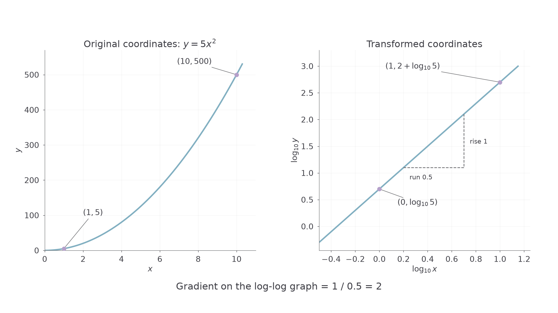
The transformed graph is a new plot of new coordinates. The original curve has not suddenly become straight on its original axes.

Change only the exponent from $2$ to $-2$. The line now slopes downwards; the coefficient stays the same.

A negative gradient is compatible with positive values of both original variables.

Exponential models from semi-log graphs

An exponential model becomes linear when you take the logarithm of the output while leaving the input unchanged.

For $y=kb^x$, take $k>0$ and $b>0$. The input $x$ may be negative, zero or positive; only $y$ is being logged. The log laws give

Now compare with $Y=mX+c$ using $X=x$, rather than $\log x$.

[DIAGRAM: asset_name: Exponential growth and decay on semi-log axes; asset_slug: exponential-log-lines; caption: Reciprocal exponential bases give opposite gradients on semi-log axes.; description: Two panels show y equals four times two to x and y equals four times one half to x on ordinary axes, then their straight lines on log base ten y against x axes. Both transformed lines have intercept log four. Their gradients are log two and negative log two.]

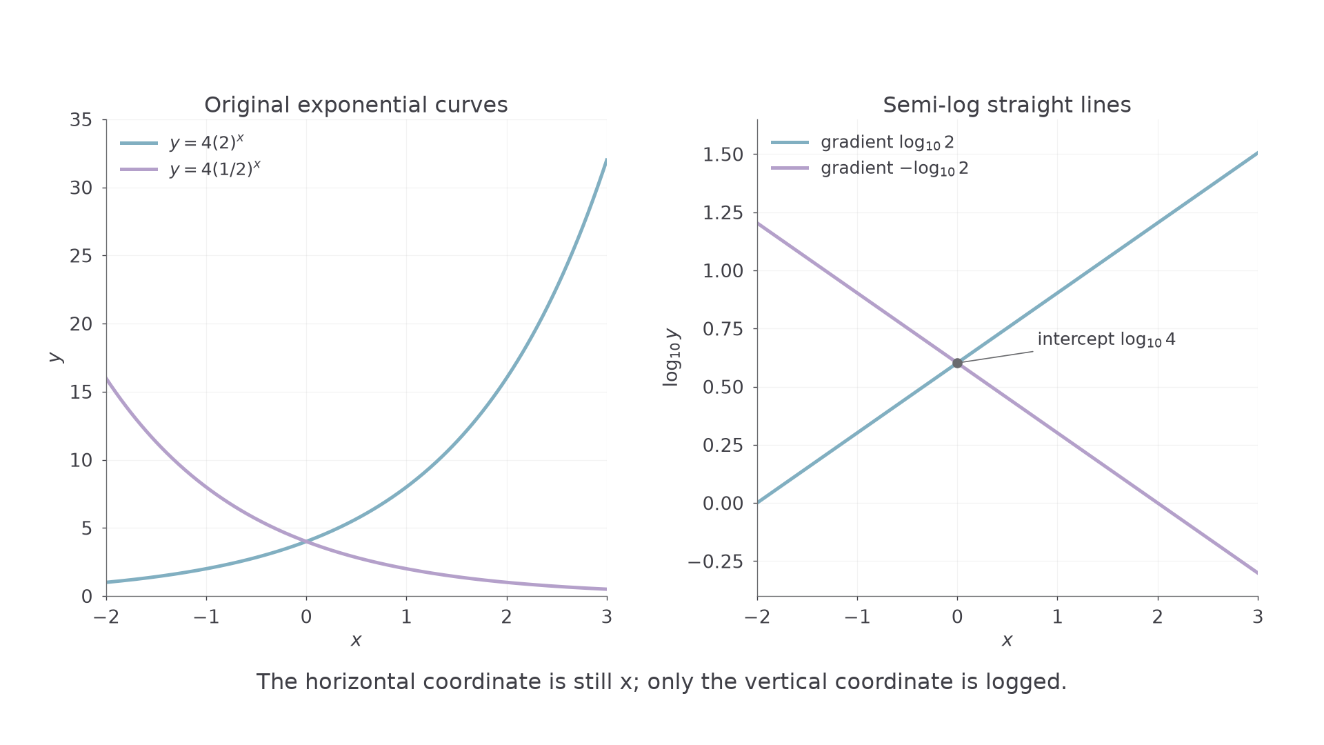
When $b>1$, $\log b>0$, giving growth. When $0<b<1$, the gradient is negative, giving decay. If $b=1$, the model is the constant $y=k$.