S1 4.1, S1 4.2 - Regression and prediction

Scatter diagrams

Can one straight line give a useful prediction when the observations do not lie exactly on it? A scatter diagram first shows whether a straight-line model is sensible.

For the pairs $(1,2),(2,3),(3,5),(4,4),(5,6)$, choose labelled numerical axes and plot all five points. For example, $(3,5)$ is three units across and five units up. Use a consistent scale on each axis, although the two axes may use different scales.

The points tend upwards from left to right and cluster around a straight line, so a positive linear relationship is plausible. Describe both the direction and the shape: a downward pattern can be linear too. A curved pattern needs care even when the overall direction is clear. Look for unusual points because a single remote observation can strongly affect a fitted line.

[DIAGRAM: asset_name: A fitted regression line and its residuals; asset_slug: regression-line-and-residuals; caption: Least squares fits vertical discrepancies for a response y; the fitted line passes through the pair of means.; description: Scatter points one-two, two-three, three-five, four-four and five-six. The fitted line is y equals one point three plus zero point nine x, drawn over the observed x range one to five. Vertical segments show residuals and the mean point three-four is marked.]

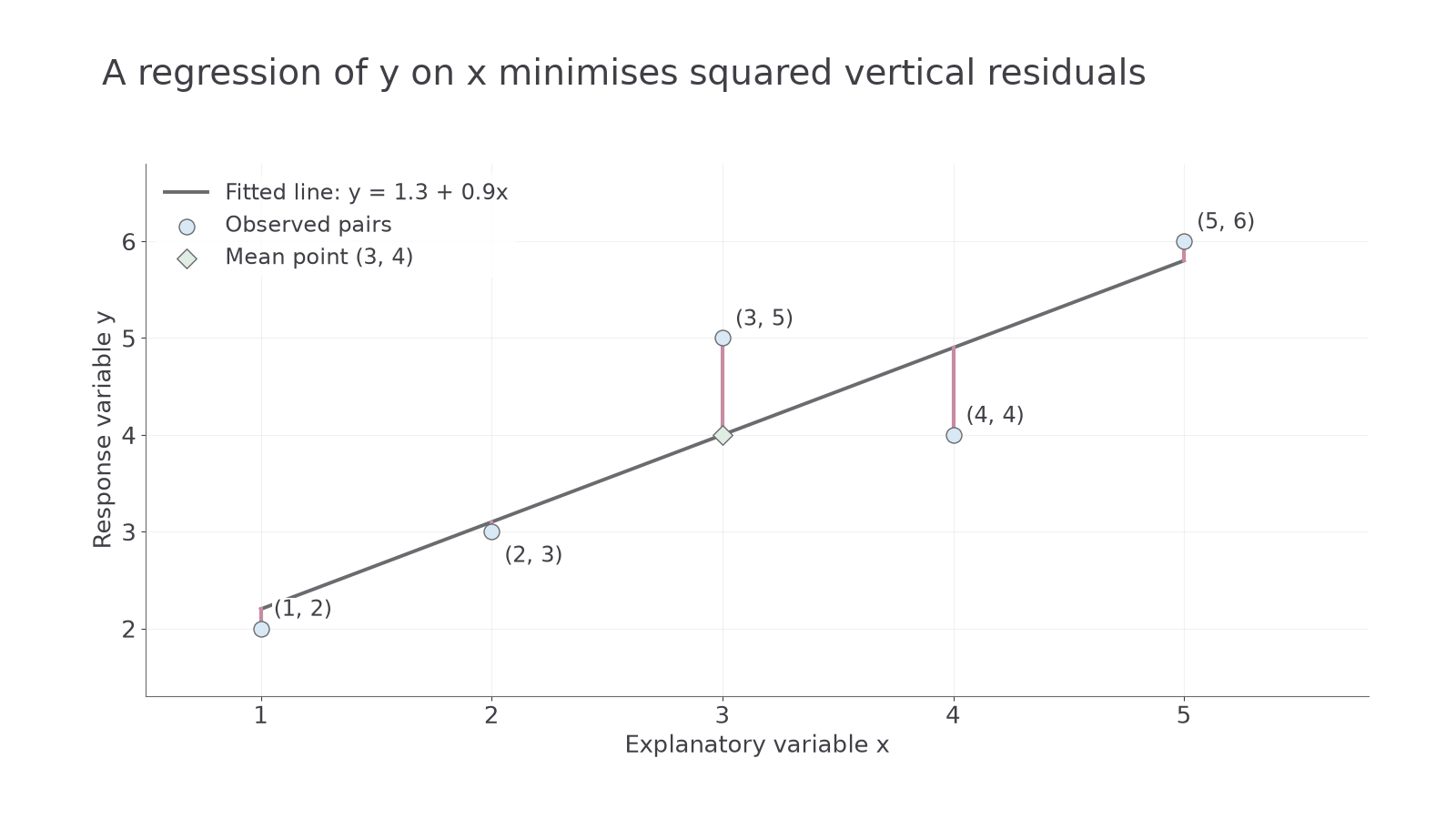
The line in the diagram is calculated from all five pairs, rather than obtained by joining the first and last points. Its calculation is taught in Part 3.

Explanatory and response variables

Before fitting a line, decide which measured quantity will be used to predict the other.

If study time $h$ is used to predict a quiz score $s$, fit the regression of $s$ on $h$. Put $h$ horizontally and $s$ vertically. An equation $s=18+4h$ predicts an increase of $4$ score points per extra hour of study, on average under the model. It does not say every student gains exactly four points or establish that changing study time causes the whole association.

The regression of $y$ on $x$ minimises the sum of squared vertical residuals, where a residual is observed response minus fitted response:

Squaring makes discrepancies in either direction contribute positively and gives larger discrepancies more weight. The regression of $x$ on $y$ instead predicts $x$ and minimises discrepancies in that response. Usually these are different lines: rearranging one equation does not calculate the other regression. No derivation of least squares is required in S1.

If the question asks for a prediction of score from time, use the score-on-time line. If time is to be predicted from score, the appropriate direction must be fitted to the data. Variable letters can be anything; read the context and the phrase “response on explanatory variable”.

Least-squares line from summaries

The line's gradient depends on how the two variables vary together relative to the spread of the explanatory variable.

The equivalent form $y-\bar y=b(x-\bar x)$ shows that the line passes through $(\bar x,\bar y)$. If every explanatory value is the same, $S_{xx}=0$ and these data cannot determine a regression gradient. Retain working precision until the final equation.