S1 5.1 - Normal probabilities
Use the shape, symmetry and parameters of a Normal distribution to describe continuous measurements. Standardise values and use the supplied cumulative tables to calculate probabilities in either tail or between two limits.
Shape symmetry mean and variance
Is a measurement of unusually large? That depends on the usual value and the spread: is far less surprising when measurements vary widely. A Normal model supplies both pieces of information.
Normal distribution
A Normal distribution is a continuous, bell-shaped probability distribution symmetric about its mean . We write
where is the variance and is the standard deviation.
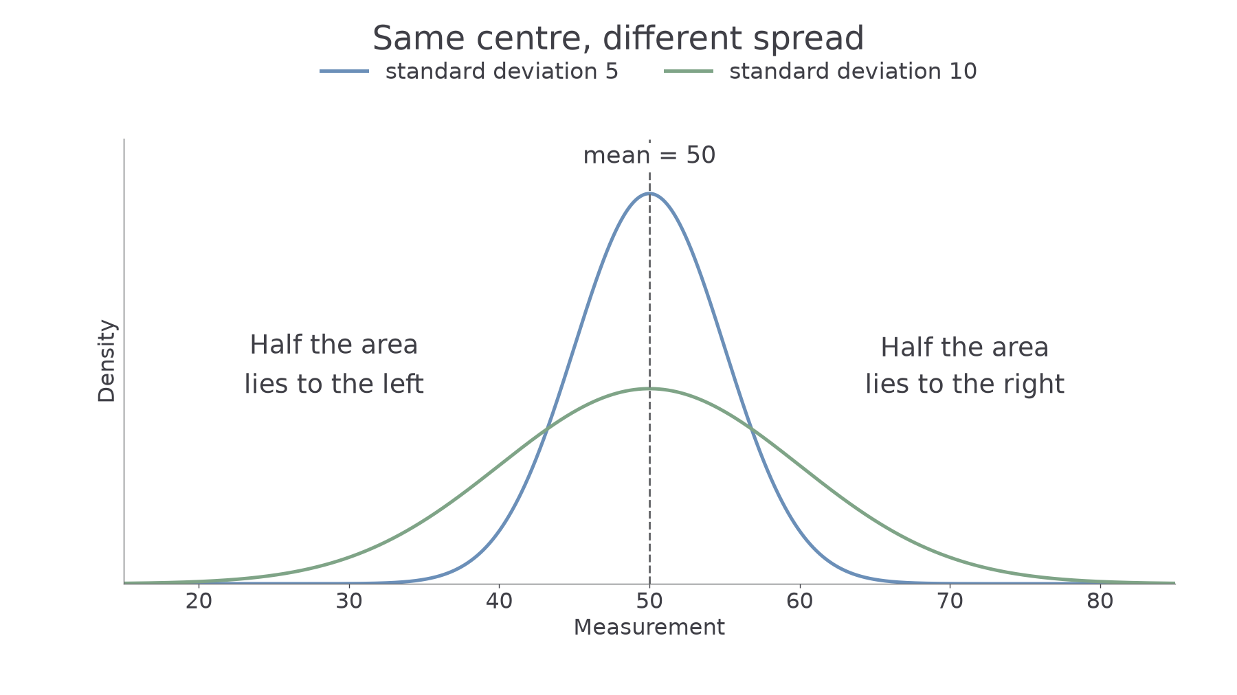
The mean, median and mode coincide at the centre. Increasing spreads the curve out and lowers its peak, while keeping the total area equal to . Half the area lies on each side of .
[DIAGRAM: asset_name: Normal centre and spread; asset_slug: s1-normal-centre-spread; caption: Both Normal curves have mean 50 and total area one. The curve with standard deviation 10 is more spread out.; description: Exact Normal curves with mean 50 and standard deviations 5 and 10, sharing a horizontal measurement axis. Their peaks align at 50. A dashed central line marks the mean, and two side labels identify one half of each distribution on either side.]
Probabilities are areas under the curve, not heights. A single exact value has zero area, so . Thus , and including or excluding interval endpoints does not change a Normal probability. This differs from a discrete distribution, where one supported value can have positive probability.
A Normal model allows values across the whole real line. For a physical quantity that cannot be negative, it is an approximation that may be useful when the impossible tail is negligible. Symmetry and a single central peak support the model; pronounced skewness or several peaks count against it. Being continuous alone is insufficient.
Watch out
In , the standard deviation is , not . The second parameter is the variance.
Read both the parameters and the meaning of a continuous probability.
Standardising a value
The useful question is how many standard deviations a measurement lies above or below its mean. Subtracting the mean removes its location; dividing by the standard deviation measures the distance in standard-deviation units.
For a model with mean and standard deviation , the value is units above the mean, or standard deviations above it. The value is the same distance below it.
Standardising a Normal variable
If , then
For a boundary , its standardised value is . Since , standardising does not reverse an inequality.
Not in the formula booklet: learn it.
The new variable is the standard Normal variable. It has no measurement units. Its mean is zero and its variance is one; every Normal model can therefore use the same probability table.
Worked example 1: a value above the mean
. Standardise the boundary , and rewrite in terms of .
Plan. Subtract from the boundary and divide by .
Answer. The boundary has ; it is standard deviations above the mean.
Check. Returning to the original scale gives .
Change only the boundary to the same distance below the mean. Its standardised value must be negative.
Worked example 2: a value below the mean
. Standardise , and rewrite .
Plan. Use the signed difference between the boundary and the mean.
Answer. The boundary has ; it is standard deviations below the mean.
Check. . A negative standardised value correctly places it to the left of the mean.
Writing the standardisation also makes the choice of scale visible. Use the standard deviation in the denominator, even when the model is given with its variance.
Cumulative probabilities from tables
The supplied Normal distribution function table gives the area to the left of a standardised boundary. It does not give the area between zero and that boundary.
Cumulative Normal probability
For ,
The booklet's table gives for nonnegative . For example, the entry beside is : that includes all the area to the left of zero as well as the area from zero to .
The table starts with . To use a negative boundary, reflect its left tail into the equal right tail at the corresponding positive boundary:
The symmetry is about zero on the standardised scale.
Continue this lesson.
You’re previewing NovaLearn without an account. Create a free account to read the rest.
Create free account