S1 5.1 - Finding Normal parameters
Work backwards from a Normal probability to a boundary, mean or standard deviation. Translate percentile conditions into signed standardised values, then solve two conditions together when both parameters are unknown.
Inverse standard Normal probabilities
Where does the lowest of a Normal distribution end? Its boundary must lie below the mean, so its standardised value must be negative. Choosing the sign is as important as finding the table entry.
A percentile is a boundary below which a stated percentage of the distribution lies. For example, the 90th percentile has cumulative probability . It leaves probability to its right.
The booklet has two useful tables. The cumulative table gives . The percentage-points table gives nonnegative such that
For example, its entry , means that lies above , not below it. Its entry , identifies the 85th percentile. If the required cumulative probability is , use and reflect the listed to .
[DIAGRAM: asset_name: Opposite ten-percent tails; asset_slug: s1-normal-inverse-signs; caption: The lowest and highest ten percent have equal areas at opposite signed standardised boundaries.; description: A standard Normal curve shades the lower 10 percent to the left of negative 1.2816 and the upper 10 percent to the right of positive 1.2816. Both signed boundaries and zero are labelled; the central 80 percent is unshaded.]
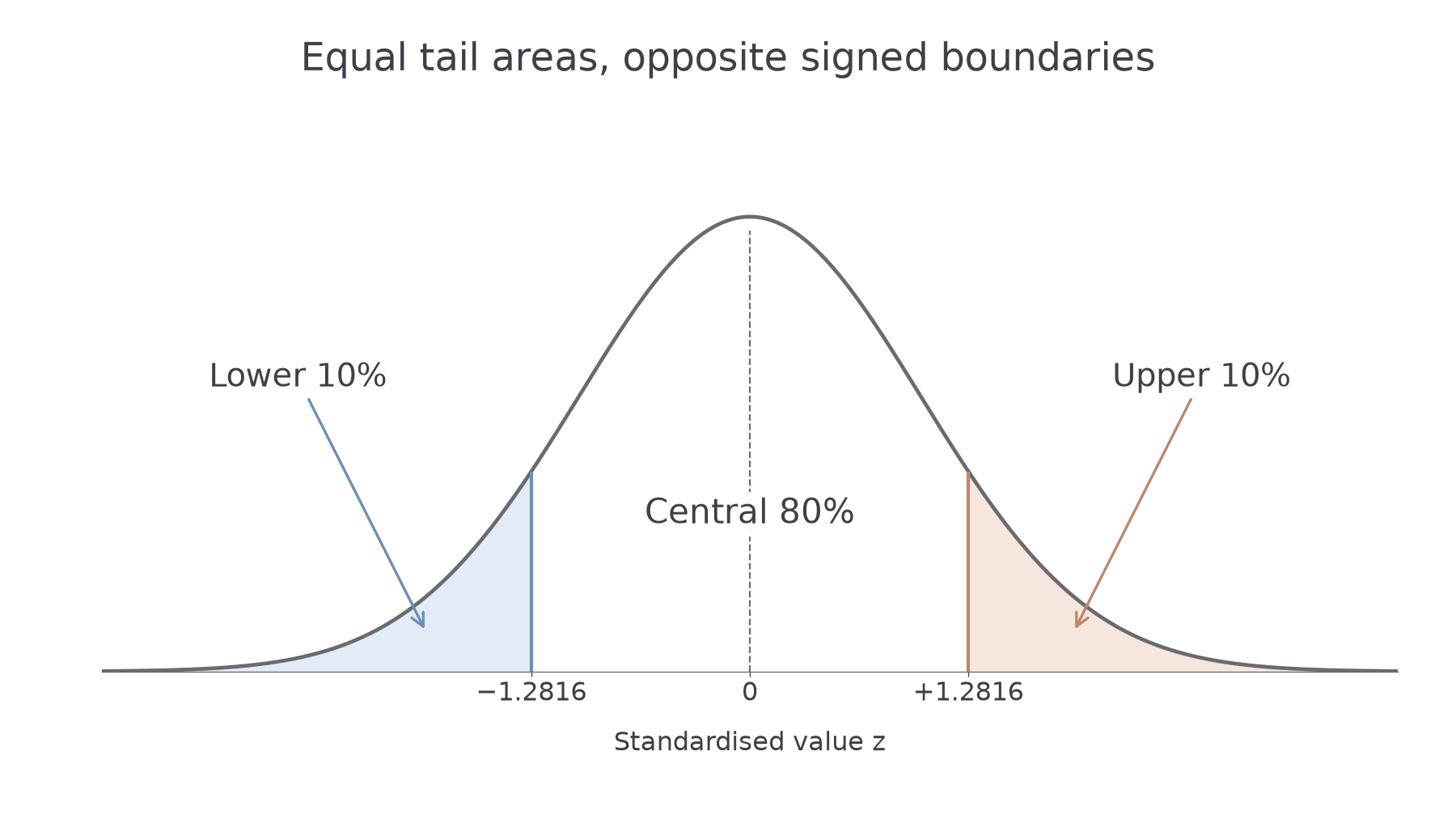
When the cumulative probability is supplied as a table entry, you can also read the cumulative table backwards: gives . No interpolation is required. A calculator inverse-Normal function usually asks for the cumulative left probability; check that convention before entering a right-tail probability.
Key idea
First locate the boundary relative to the mean. A cumulative probability below has a negative standardised boundary; one above has a positive boundary.
Use the full tabulated four decimal places for percentage points in subsequent equations. Rounding prematurely to , for example, can alter a calculated standard deviation.
Worked example 1: an upper ten-percent boundary
For , find such that .
Plan. This is exactly the right-tail convention of the percentage-points table.
Answer. .
Check. Its cumulative left probability is , so the boundary is above zero and leaves the required on its right.
Change only the side of the probability from right to left, keeping . Symmetry reverses the sign of the boundary.
Worked example 2: a lower ten-percent boundary
For , find such that .
Plan. Reflect the upper ten-percent boundary in zero.
Answer. .
Check. The boundary lies below the mean and lies above it. A positive answer would instead leave more than half the distribution to its left.
Match the requested tail before reading off a sign.
Unknown mean or standard deviation
A probability condition tells you the standardised distance of a boundary from the mean. With one unknown parameter, this gives one equation to solve.
If a boundary corresponds to standardised value , then
The second form reads naturally: boundary equals mean plus a signed number of standard deviations. To find a percentile boundary when both parameters are known, simply substitute into this form. For example, a positive adds a distance above the mean; a negative subtracts a distance.
Recovering a parameter
The standard deviation must be positive. A condition at the median has : it gives but supplies no information about .
These are rearrangements of standardisation, not separately provided formulae.
Find the signed first. Do not treat a percentage or probability as the standardised value.
Worked example 3: finding a mean
and . Find .
Plan. An upper tail of puts the boundary standard deviations above the mean.
Answer. , to three significant figures.
Check. . The boundary exceeds the mean, which agrees with the small upper-tail probability.
Keep the boundary and probability fixed, but change which parameter is known. Now the mean is given and the scale must be found.
Worked example 4: finding a standard deviation
and . Find .
Plan. Use the same positive percentage point, then divide the distance above the mean by it.
Answer. , to three significant figures.
Check. The result is positive, and . Dividing by instead would use the wrong scale.
Continue this lesson.
You’re previewing NovaLearn without an account. Create a free account to read the rest.
Create free account