6.4.3(d)-(h) - Activity, half-life, decay and dating

Activity and decay constant

A radioactive source contains many unstable nuclei. You cannot predict which particular nucleus will decay next, but you can predict the average rate at which a large number of nuclei decay.

If a sample has a large number $N$ of undecayed nuclei, the activity is higher when $N$ is larger. It is also higher for an isotope whose nuclei have a larger chance of decaying in each second. That probability per unit time is represented by the decay constant.

For a sample containing $N$ undecayed nuclei:

This equation is physically sensible: doubling the number of undecayed nuclei doubles the average number of decays per second, and using an isotope with twice the decay constant also doubles the activity. Since $A$ is a positive rate of decay, the rate of change of $N$ itself is negative:

The minus sign means the number of undecayed nuclei is decreasing. The activity is the magnitude of that decrease: $A=-\frac{dN}{dt}$.

An amount of radioactive isotope can be converted to a number of nuclei using:

where $n$ is the amount of substance in mol and $N_A = 6.02 \times 10^{23}\ \mathrm{mol}^{-1}$.

Worked example: a sample contains $3.0 \times 10^{-10}\ \mathrm{mol}$ of an isotope with decay constant $2.5 \times 10^{-4}\ \mathrm{s}^{-1}$. Find its activity.

First convert amount of substance to number of nuclei:

Then use $A = \lambda N$:

The answer is large because a becquerel is only one decay per second; many radioactive samples contain enormous numbers of nuclei.

Probability over a time interval

A probability lies between 0 (impossible) and 1 (certain). For a short interval $\Delta t$, an undecayed nucleus has decay probability approximately $p=\lambda\Delta t$, provided $\lambda\Delta t\ll1$. The exact probability of decay during time $t$ is $1-e^{-\lambda t}$; the probability of surviving is $e^{-\lambda t}$. The decay constant is a rate, so it is not itself a dimensionless probability and can exceed $1\,\mathrm{s^{-1}}$.

For example, with $\lambda=0.020\,\mathrm{s^{-1}}$, the probability of decay in the next $5.0\,\mathrm{s}$ is $1-e^{-0.10}=0.0952$, about 9.5%. A nucleus which has survived for a long time still has this same probability during its next 5.0 s; it does not become “due” to decay. In 1000 independently decaying nuclei, about 95 decays are expected in that interval, but the observed count varies.

Half-life and exponential shape

Half-life is a way of describing the same decay process without counting every nucleus. It is not the time for all the nuclei to decay. It is the time for the number of undecayed nuclei, and therefore the activity, to halve.

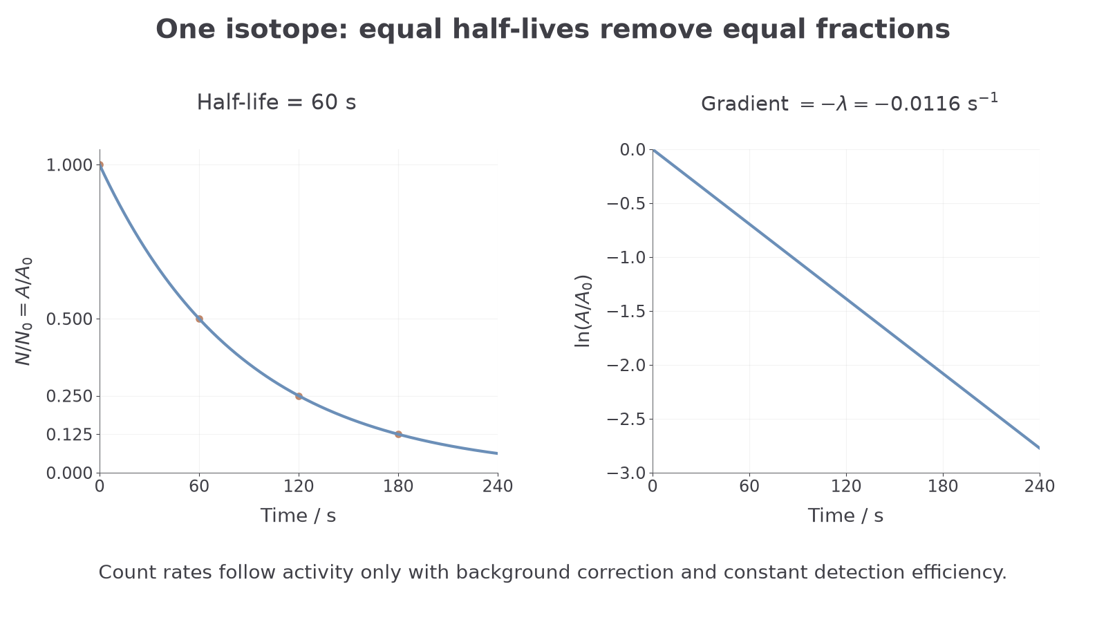
Because $A = \lambda N$, activity and the number of undecayed nuclei of one isotope halve together. A measured count rate follows this pattern only after background correction and with unchanged detection efficiency and geometry. After one half-life, $\frac{N}{N_0}=\frac12$; after two half-lives, $\frac{N}{N_0}=\frac14$; after three, $\frac{N}{N_0}=\frac18$.

The relationship between half-life and decay constant is:

You can see where this comes from by using the exponential model. If half the nuclei remain:

Cancel $N_0$ and take natural logs:

so:

A large decay constant gives a short half-life. A small decay constant gives a long half-life. That inverse link is a common source of errors: high activity is not the same idea as long half-life.

[DIAGRAM: asset_name: 6.4.3(d)-(h) - Activity, half-life, decay and dating - diagram 1; asset_slug: 6_04_3b_activity_half_life_exponential_decay_and_dating__diagram_01; recommended_method: drawn_physics; description: Analytic exponential and ln ratio share seconds axis; half-life 60 s and gradient −0.0116 s⁻¹ agree.; caption: Exponential decay with a 60 s half-life becomes a straight line when the natural logarithm of the activity ratio is plotted.]

Using the decay equations

The same exponential form can be written for undecayed nuclei or for activity:

Here $N_0$ and $A_0$ are the initial number of undecayed nuclei and initial activity. The two equations have the same shape because activity is proportional to the number of undecayed nuclei.

You can also use the half-life version:

This is often faster when the time is an exact number of half-lives. Use the natural-log version when the remaining fraction is not a simple power of a half.

Worked example 1: a medical tracer has half-life $110\,\mathrm{min}$. Find the time for its activity to fall to $30\%$ of its initial value.

Use the activity ratio:

Find $\lambda$ in $\mathrm{min}^{-1}$ because the answer is wanted in minutes:

Then:

Take natural logs:

The negative sign matters: $\ln(0.30)$ is negative, and time must be positive.

Worked example 2: a pure radioactive isotope has half-life $2.0\,\mathrm{h}$, molar mass $0.060\,\mathrm{kg}\,\mathrm{mol}^{-1}$, and initial activity $250\,\mathrm{MBq}$. Estimate the initial mass of isotope present.

Convert the half-life to seconds:

Use $A = \lambda N$:

Convert nuclei to moles and then mass:

This type of chain is why unit discipline matters. Use seconds with $\mathrm{Bq}$ unless you have deliberately expressed $\lambda$ in another time unit.

Logarithmic scales and decay plots

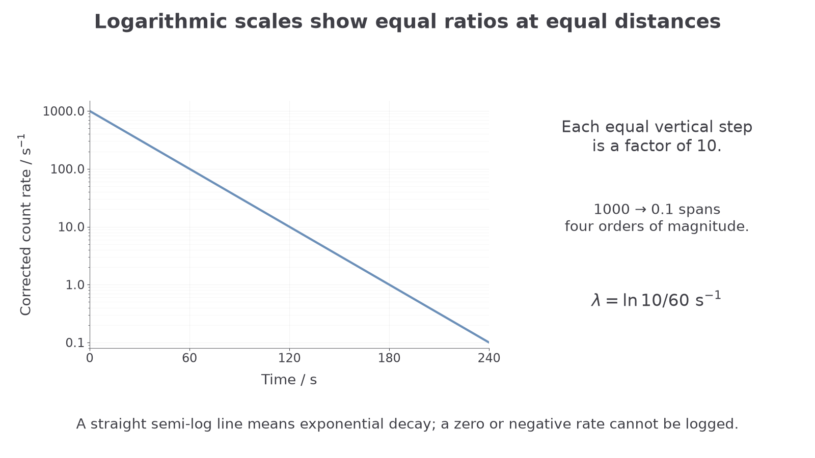
A linear vertical scale assigns equal distances to equal differences. A logarithmic scale assigns equal distances to equal ratios: marks at $0.1,1,10,100,1000\,\mathrm{s^{-1}}$ are equally spaced and span four orders of magnitude. This displays a large range of corrected count rates clearly. Halfway between 10 and 100 on a log scale is $\sqrt{10\times100}=31.6$, not 55. Zero and negative values cannot appear on a logarithmic axis; a late background-subtracted value near zero cannot safely be logged.

Let $C$ denote background-corrected count rate. With fixed geometry, $C=C_0e^{-\lambda t}$. Taking natural logarithms of a dimensionless ratio gives

A straight line of $\ln(C/C_0)$ against $t$ supports an exponential model; its gradient is $-\lambda$. If instead the plot uses $\log_{10}(C/\mathrm{s^{-1}})$, then

The base-10 gradient is $-\lambda/\ln10$, not $-\lambda$. Read two widely separated points on the best-fit line, not just adjacent measured points.

Worked example: a semi-log plot falls from $1000\,\mathrm{s^{-1}}$ to $10\,\mathrm{s^{-1}}$ in 120 s. This is two equal decade intervals, giving base-10 gradient $(1-3)/120=-1/60\,\mathrm{s^{-1}}$. Hence $\lambda=\ln10/60=0.0384\,\mathrm{s^{-1}}$ and $t_{1/2}=\ln2/\lambda=18.1\,\mathrm{s}$. The straight line represents equal fractional loss in equal times, even though the raw rate decreases along a curve.

[DIAGRAM: asset_name: Logarithmic scales for radioactive decay; asset_slug: 6_04_3b_logarithmic_scales__diagram_04; recommended_method: drawn_physics; description: A semi-log graph of corrected rate from 1000 to 0.1 per second over 240 s, with equal decade spacing. Each factor-of-ten decrease takes 60 s.; caption: Adjacent labelled ticks on this logarithmic count-rate axis differ by a factor of ten.]