1.1.3 - Analysing experimental data

From Results To Conclusions

Analysis is the stage where raw observations become evidence. A raw result is what was read or observed directly: a stopwatch reading, a voltmeter reading, a measurement on a ruler, or a qualitative observation such as "the oscillations became smaller". A processed result is obtained from raw results: a mean, a calculated value, a graph coordinate, a gradient, an intercept, or a comparison.

Good analysis keeps those two types of evidence separate. A statement such as "the line goes up" is qualitative. A statement such as "the gradient is $1.8\,\mathrm{m}\,\mathrm{s}^{-1}$" is quantitative. OCR questions often require both: the numerical processing gives a value, and the interpretation explains what that value means.

A useful analysis route is:

1. Record the raw readings with units and consistent precision.
2. Process the readings using the correct mathematical operation.
3. Look for a pattern, relationship, gradient, intercept, or comparison.
4. State a conclusion that follows from the processed evidence.

The conclusion must be valid for the data you actually have. If the processed values show an increasing straight-line trend, it is fair to say the dependent variable increases linearly with the independent variable over the tested range. It is not fair to claim the same relationship for all possible values unless you have a model and evidence for that wider claim.

Here, $x_1, x_2, \ldots$ are repeated readings of the same quantity and $n$ is the number of readings. Repeats reveal the spread and possible anomalies, so the precision and repeatability of the measurements can be assessed. When the variation is random, the mean gives a better estimate because high and low fluctuations tend to offset; it does not remove systematic error. Later evaluation lessons deal more fully with anomalies and confidence in conclusions; here the focus is on processing and interpreting the data.

Worked example: processing repeated readings

A student measures the time for one event three times:

$1.18\,\mathrm{s}$, $1.21\,\mathrm{s}$, $1.19\,\mathrm{s}$

The mean time is

The raw times were recorded to $0.01\,\mathrm{s}$, so a sensible processed value is

The analysis does not stop at the arithmetic. A valid conclusion would be something like: "For this set of repeats, the best estimate of the time is $1.19\,\mathrm{s}$." It would be too strong to say the exact time is $1.193333\ldots s$, because the apparatus and repeated readings do not justify that precision.

Significant Figures

Significant figures are the meaningful digits in a measured or calculated value. They are not decoration. They tell the reader how much precision the data can support.

For example:

• $0.00470$ has three significant figures: $4$, $7$, and the final $0$.
• $3.20$ has three significant figures.
• $3.2$ has two significant figures.
• $2.30 \times 10^{2}$ clearly has three significant figures, while $2.3 \times 10^{2}$ has two.

OCR expects calculated results to be reported to a precision justified by the data. A calculator display is not an answer. If the least precise measured input has two significant figures, a final answer with six significant figures usually exaggerates what the experiment can support.

For ordinary OCR calculation marking, extra significant figures are not penalised; use any explicit precision instruction. Choosing suitable reporting precision is itself assessed when the question specifically asks for it.

The most useful habits are:

• keep extra digits during intermediate working;
• round only the final answer unless the question asks otherwise;
• use standard form when a trailing zero could be ambiguous;
• give units with physical quantities;
• keep raw readings of the same quantity to a consistent number of decimal places where the apparatus allows it.

Worked example: avoiding calculator precision

A student calculates a value from

The calculator gives

The value $0.032$ is quoted to two significant figures and is the least precise number in the calculation. A suitable final answer is therefore

or, if a unit is required in the context, $26$ with that unit. Writing $26.4375$ would imply much more precision than the measurements justify.

Be careful: this is a reporting rule for the final processed result, not permission to throw away information early. If $26.4375$ is needed in a later step, keep the unrounded value in the calculator and round only the final result.

Plotting Experimental Graphs

A graph is a calculation tool, not just a picture of the data. It can show whether a relationship is linear, whether a trend is increasing or decreasing, and whether a physical value can be found from a gradient or intercept.

The usual convention is:

• put the independent variable on the horizontal axis;
• put the dependent variable on the vertical axis;
• label each axis with a quantity and a unit;
• choose a scale that uses the plotting area sensibly and is easy to read;
• plot data points accurately, usually with small crosses;
• draw a line or curve of best fit that represents the trend, not a dot-to-dot join.

Axis labels should distinguish the quantity from the unit. These are good labels:

• $t /\mathrm{s}$
• $V /\mathrm{V}$
• $L /\mathrm{m}$
• $T^{2} / \mathrm{s}^{2}$

These are poor labels:

• seconds
• volts
• length
• $T^{2}$

The poor labels either give only the unit or omit the unit. Choose evenly spaced scale intervals such as 1, 2 or 5 times a power of ten. The scale need not start at zero if a restricted range makes the data clearer; show the values honestly and do not infer an intercept from an unlabelled axis edge.

For a proposed relationship $y=kx^2$, plot $y$ against $x^2$, not $x$, to test for a straight line through the origin. If $x$ is in metres, the horizontal label is $x^2/\mathrm{m}^2$. A straight line with a non-zero intercept shows a linear relationship between the plotted variables, but does not establish direct proportionality.

If uncertainties are supplied for plotted values, show them with error bars. An error bar is not a new data point; it shows the range within which the measured value is expected to lie according to the uncertainty information supplied. For this lesson, the key analysis idea is that error bars affect what lines of fit are acceptable and therefore what gradients and intercepts are reasonable.

Worked example: choosing axes and labels

A student changes the length $L$ of a pendulum and calculates $T^{2}$ from measurements of the time period $T$. The instruction is to plot $T^{2}$ against $L$.

The correct axes are:

• horizontal axis: $L /\mathrm{m}$
• vertical axis: $T^{2} / \mathrm{s}^{2}$

The phrase "plot $Y$ against $X$" means put $Y$ on the vertical axis and $X$ on the horizontal axis. The units follow from the quantities: if $T$ is measured in seconds, then $T^{2}$ has unit $\mathrm{s}^{2}$.

Gradients And Intercepts

Many experimental relationships can be written or rearranged into the straight-line form

Here, $y$ is the vertical-axis quantity, $x$ is the horizontal-axis quantity, $m$ is the gradient, and $c$ is the vertical-axis intercept. The intercept is the value of $y$ when $x = 0$, if the line can sensibly be extended to the vertical axis.

The units of a gradient are the vertical-axis unit divided by the horizontal-axis unit. If the graph is $s /\mathrm{m}$ against $t /\mathrm{s}$, the gradient unit is $\mathrm{m} \mathrm{s}^{-1}$. If the graph is $F /\mathrm{N}$ against $x /\mathrm{m}$, the gradient unit is $\mathrm{N} \mathrm{m}^{-1}$.

When finding a gradient from experimental data, use two well-separated points on the line of best fit. Do not simply choose two plotted data points unless they happen to lie exactly on the fitted line. A large gradient triangle reduces the percentage uncertainty in reading the coordinates. When the horizontal axis is time, the gradient gives a rate of change: a straight displacement–time graph has constant velocity, and a straight velocity–time graph has constant acceleration. Read the physical meaning from the plotted quantities, rather than calling every gradient a speed.

Worked example: gradient and intercept from a fitted line

A graph of $s /\mathrm{m}$ against $t /\mathrm{s}$ has a straight line of best fit. Two points on the line are:

• $(t, s) = (0.20\,\mathrm{s}, 0.54\,\mathrm{m})$
• $(t, s) = (0.90\,\mathrm{s}, 1.80\,\mathrm{m})$

The gradient is

To find the intercept, use $y = mx + c$, so

Using the first point on the line:

The gradient has units $\mathrm{m} \mathrm{s}^{-1}$ because it is a change in distance divided by a change in time. The intercept has units $\mathrm{m}$ because it is a value on the vertical axis.

Uncertainty-Aware Analysis

Uncertainty-aware analysis means using the precision of the data honestly when you calculate and conclude. This lesson only needs the analysis side: significant figures, error bars where supplied, and the effect of best-fit and worst-fit lines on gradients or intercepts. A later evaluation lesson deals more fully with precision, accuracy, limitations and improvements.

If a graph has a best-fit line and a worst acceptable line, an OCR-style estimate of uncertainty in the gradient is often found from the difference between the two gradient values:

Similarly, an uncertainty in an intercept can be estimated from the difference between the intercept from the best-fit line and the intercept from the worst acceptable line:

For supplied vertical error bars with negligible horizontal uncertainty, a candidate line must pass through every relevant error bar to count as acceptable. Choose the steepest or shallowest acceptable line that differs most from the best-fit gradient; a line that misses a bar is not acceptable simply because it passes through the first and last bars. If no straight line can pass through the bars, investigate the uncertainty estimates, anomalous points or the straight-line model.
[DIAGRAM: asset_slug: 1_01_3_analysis_graphs_and_uncertainties__diagram_01; caption: Best-fit and shallowest acceptable displacement–time lines cross every uncertainty bar. Their gradients give velocity estimates.; description: Displacement against time: best-fit and shallowest acceptable lines intersect every uncertainty bar; the gradient is a velocity.]

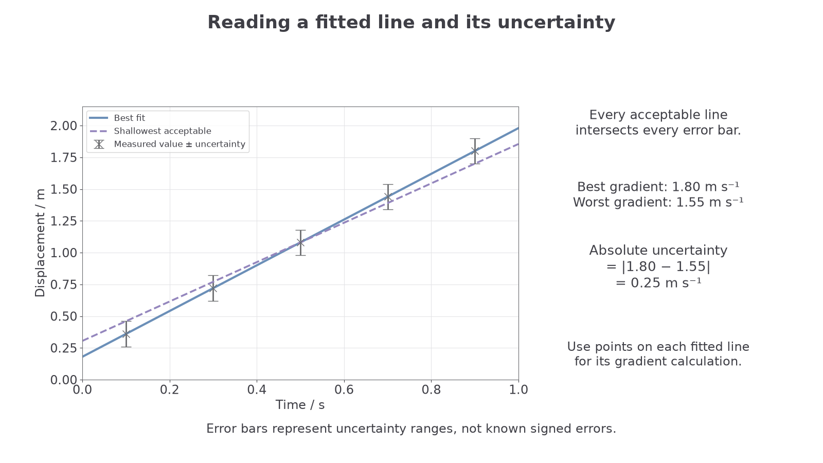
The uncertainty should be quoted as a positive value. The final value and the uncertainty should be presented with compatible precision. For example, $1.82 \pm 0.14$ uses the same decimal place for the central value and the absolute uncertainty.

Worked example: using a worst acceptable line

A graph gives:

• best-fit gradient $m_{\mathrm{best}} = 1.82\,\mathrm{m}\,\mathrm{s}^{-1}$
• worst acceptable gradient $m_{\mathrm{worst}} = 1.68\,\mathrm{m}\,\mathrm{s}^{-1}$

The uncertainty in the gradient is

So the gradient can be reported as

This means the graph analysis supports a range from about $1.68\,\mathrm{m}\,\mathrm{s}^{-1}$ to $1.96\,\mathrm{m}\,\mathrm{s}^{-1}$. If an accepted value of $1.75\,\mathrm{m}\,\mathrm{s}^{-1}$ is being compared with the result, it is consistent with this graph result. If the accepted value were $2.20\,\mathrm{m}\,\mathrm{s}^{-1}$, it would not be consistent with this uncertainty range.

Notice the boundary of the claim. A good conclusion is not "the accepted value is definitely correct". A better conclusion is "the accepted value is consistent with the value from the graph, within the uncertainty estimated from the best and worst acceptable lines."