5.1.4(e)-(i) - Kinetic theory of ideal gases

Pressure From Particle Motion

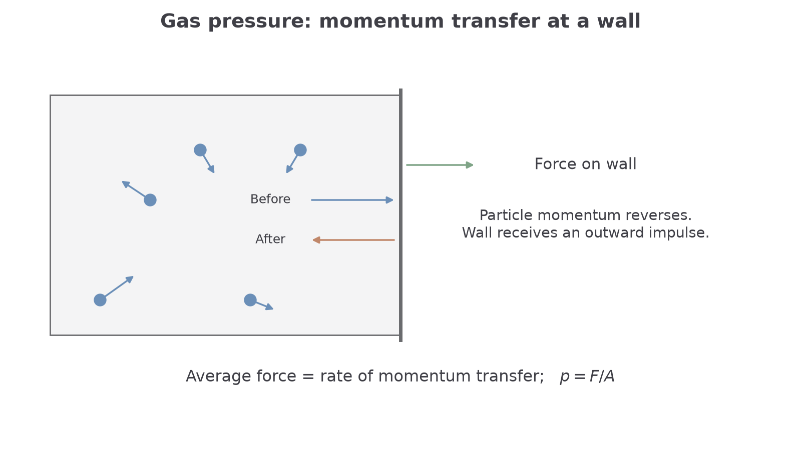
In the ideal-gas model, gas particles move rapidly and randomly. They collide elastically with the walls of their container, so each collision changes the particle's momentum and gives an impulse to the wall. A huge number of these collisions every second produces a steady average force on the wall, and pressure is force per unit area.

OCR gives the kinetic-theory pressure equation as:

You may see the OCR data booklet print this compactly as $pV = \frac{1}{3}Nmc^2$. In this lesson, read that $c^2$ as the mean square speed. The root mean square speed is:

The full derivation of $pV = \frac{1}{3}Nm\overline{c^2}$ is not required by OCR. What matters is the physical meaning: greater particle number, greater particle mass, or greater mean square speed gives more momentum transfer to the walls. At fixed $N$, $m$, and $V$, increasing the mean square speed increases the pressure.

Worked example: finding r.m.s. speed from the pressure equation

A sample of gas has pressure $1.20 \times 10^5\ \text{Pa}$, volume $2.00 \times 10^{-3}\ \mathrm{m^3}$, $5.00 \times 10^{22}$ particles, and particle mass $4.65 \times 10^{-26}\ \mathrm{kg}$. Estimate the r.m.s. speed.

Start with:

Rearrange:

Substitute:

So:

The r.m.s. speed is about $560\,\mathrm{m}\,\mathrm{s}^{-1}$.

[DIAGRAM: asset_slug: 5_01_4b_kinetic_theory_of_ideal_gases__diagram_01; description: The wall reverses a molecule’s normal momentum component; repeated impacts produce pressure.; caption: Collisions reverse the normal component of molecular momentum and produce gas pressure.]

Rms Speed And Distributions

A gas does not have one single molecular speed. Even at a fixed temperature, some particles are slow, many have middle-range speeds, and a few are much faster. That is why OCR distinguishes between mean square speed and r.m.s. speed.

If a small sample has particle speeds $c_1, c_2, c_3,\ldots$, then:

The order of operations matters: square the speeds first, find the mean of those squares, then take the square root. Do not take the ordinary arithmetic mean of the speeds.

Worked example: a small speed sample

Four gas particles have speeds $220\,\mathrm{m}\,\mathrm{s}^{-1}$, $340\,\mathrm{m}\,\mathrm{s}^{-1}$, $430\,\mathrm{m}\,\mathrm{s}^{-1}$, and $510\,\mathrm{m}\,\mathrm{s}^{-1}$.

The arithmetic mean speed would be $375\,\mathrm{m}\,\mathrm{s}^{-1}$, but that is not the r.m.s. speed. R.m.s. speed is larger here because it gives extra weight to higher speeds through the squaring step.

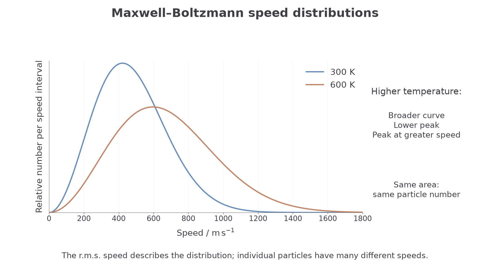
A Maxwell-Boltzmann distribution shows how the speeds of particles are spread out in a gas. OCR expects the general characteristics, not the equation for the curve:

• the curve starts at zero speed and never extends to negative speed, because speed is a magnitude
• it rises to a peak at the most probable speed
• it has a long tail at high speeds because a small number of particles move much faster than the peak speed
• increasing the temperature shifts the distribution to higher speeds, broadens it, and lowers the peak
• for the same gas sample, the total area under the curve represents the total number of particles

At one temperature, $c_{\rm rms}$ is not the most probable speed and not the ordinary mean speed. It is the speed linked directly to the particles' average kinetic energy.

[DIAGRAM: asset_slug: 5_01_4b_kinetic_theory_of_ideal_gases__diagram_02; description: Equal-area Maxwell–Boltzmann distributions at 300 K and 600 K: heating broadens the distribution and shifts its peak.; caption: Maxwell–Boltzmann distributions at 300 K and 600 K have equal areas. Heating broadens the distribution and shifts its peak.]