6.2.3 - Uniform electric fields and parallel plates

The Uniform Field Model

A uniform electric field has the same electric field strength and the same direction at every point in the region being considered. Between two large, oppositely charged, parallel plates, the central region is a good model of a uniform field. Near the plate edges the field lines spread out, so the field is no longer perfectly uniform; OCR questions often tell you to ignore these end effects.

The direction of an electric field is defined as the direction of the force on a positive test charge. So field lines go from the positive plate to the negative plate. In a uniform plate field they are drawn straight, parallel, equally spaced, and perpendicular to the plates.

[DIAGRAM: asset_name: 6.2.3 - Uniform electric fields and parallel plates - diagram 1; asset_slug: 6_02_3_uniform_electric_fields_and_parallel_plates__diagram_01; recommended_method: drawn_physics; caption: The uniform field points from the positive plate to the negative plate as potential decreases.; description: Uniform central field points from positive to negative plate; potential falls linearly with distance along the field.]

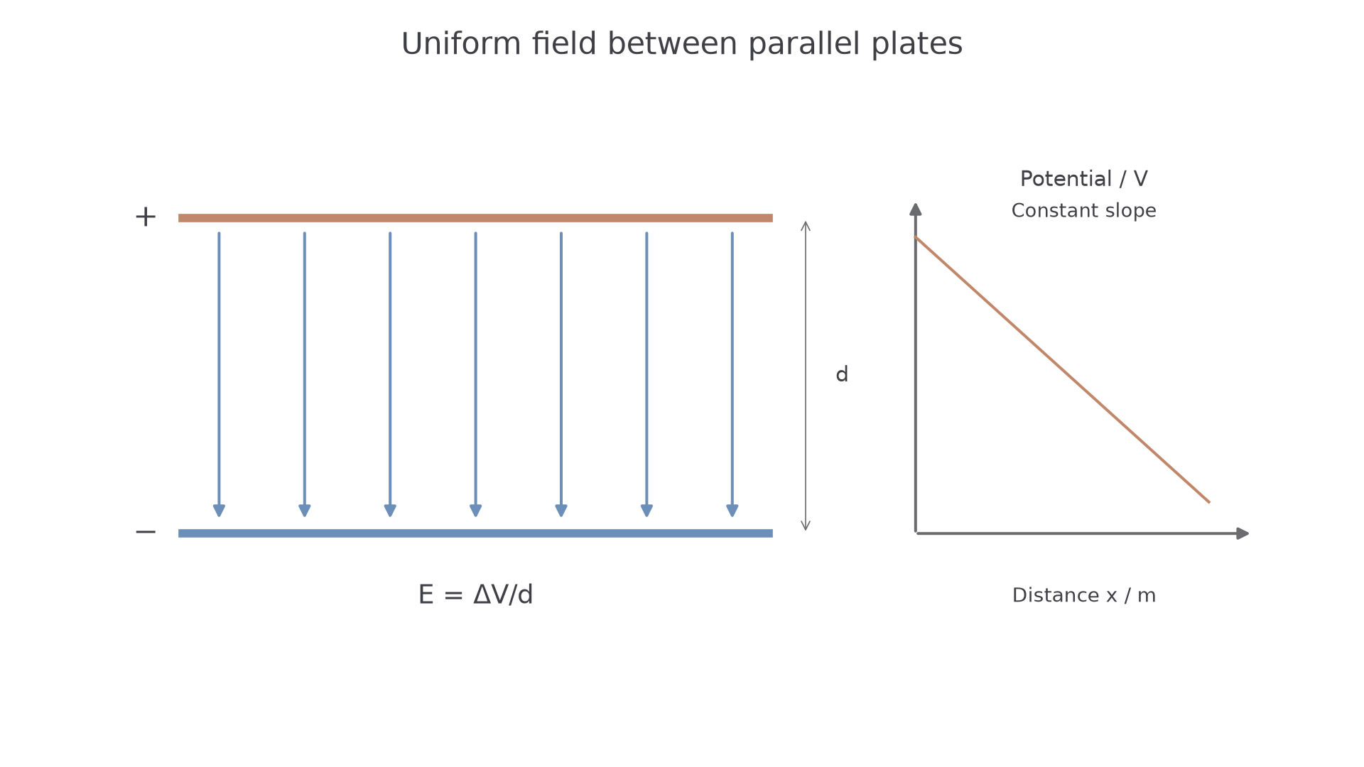
For a uniform electric field between plates:

Here $E$ is electric field strength in $\text{V m}^{-1}$, $V$ is the potential difference between the plates in volts, and $d$ is the plate separation in metres. The same field strength may also be written in $\text{N C}^{-1}$, because $E = F/q$. These two units are equivalent.

The equation says that the same p.d. spread across a smaller distance gives a stronger field. It does not mean that $d$ is the distance from a charge to one plate. In this formula, $d$ is the separation between the two plates.

Worked example: field strength between plates

Two plates have a p.d. of $2.4\ \text{kV}$ and are separated by $8.0\ \text{mm}$.

Convert first:

The field direction is from the positive plate towards the negative plate. A positive particle would be forced in that direction; an electron would be forced in the opposite direction.

Parallel-Plate Capacitance

The same two plates can also act as a capacitor. A parallel-plate capacitor stores charge on two conducting plates separated by an insulating gap. Its capacitance depends on the plate area, the separation, and the permittivity of the material between the plates.

For plates of overlapping area $A$, separated by distance $d$, with vacuum or air between them:

Here $\varepsilon_0$ is the permittivity of free space:

For a dielectric material between the plates, OCR uses:

In this equation $\varepsilon$ is the absolute permittivity of the material, and $\varepsilon_r$ is the relative permittivity. Relative permittivity has no unit. In this specification you need to use $\varepsilon_r$ in calculations and understand that it increases the capacitance compared with air or vacuum; you are not expected to explain the microscopic reason why.

[DIAGRAM: asset_name: 6.2.3 - Uniform electric fields and parallel plates - diagram 2; asset_slug: 6_02_3_uniform_electric_fields_and_parallel_plates__diagram_02; recommended_method: drawn_physics; caption: A parallel-plate capacitor has a facing plate area, a perpendicular gap and a dielectric between the plates.; description: Parallel-plate capacitor: overlapping facing area A, perpendicular gap d and dielectric permittivity.]

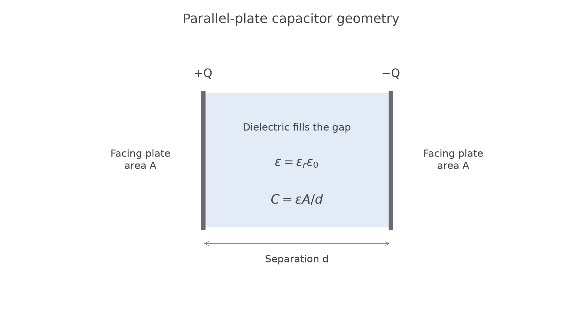
The dependencies are worth saying in words:

• larger plate area $A$ gives larger capacitance, because more charge can be stored for the same p.d.
• larger separation $d$ gives smaller capacitance
• larger permittivity $\varepsilon$, or larger $\varepsilon_r$, gives larger capacitance

Worked example: using a dielectric

A parallel-plate capacitor has plate area $4.0 \times 10^{-3}\ \text{m}^2$ and separation $0.50\ \text{mm}$. First find its capacitance in air:

If a dielectric with $\varepsilon_r = 3.2$ fills the gap, then

The geometry has not changed. The increased capacitance comes from the larger permittivity in the gap.

Linking Field and Capacitance

In a parallel-plate problem, the same geometry may appear in two equations:

The first equation tells you about the field in the space between the plates. The second tells you about how much charge the plates store for a given p.d. The bridge to earlier capacitor work is the definition of capacitance:

So a typical OCR-style chain might be:

1. use $E = V/d$ to find the p.d. between the plates
2. use $C = \varepsilon A/d$ to find the capacitance
3. use $Q = CV$ to find the charge on one plate

Worked example: idealised storm-cloud model

A region of cloud is modelled as two circular parallel plates. The effective plate diameter is $18\ \text{km}$, the separation is $2.5\ \text{km}$, and the electric field strength between the regions is $3.0 \times 10^5\ \text{V m}^{-1}$. Assume the permittivity is $\varepsilon_0$.

First find the p.d.:

The radius is $9.0\ \text{km} = 9.0 \times 10^3\ \text{m}$, so