2.1.2 - SI units, prefixes and graph labels

Base quantities and base units

A physical quantity is something that can be measured. The 2.1.2 list uses S.I. base quantities as the starting point for the units used throughout the specification.

For this lesson, learn the six base quantities named in the specification:

The symbol is not optional decoration. $\mathrm{m}$ means metre when it is the unit symbol for length; $\mathrm{mol}$ means mole; $\mathrm{A}$ means ampere. A numerical answer without its unit is usually incomplete because the same number can mean very different things.

There is one boundary detail to keep tidy. The full international S.I. system also has luminous intensity as a base quantity, with unit candela, but this 2.1.2(a) outcome does not list it. In this lesson, answer using the list above.

Derived units from base units

Most useful physics units are derived units. They are made by combining base units according to the definition of the quantity or according to an equation.

The specification gives momentum and density as examples in this section. Without teaching the later topics in detail, you can see how their units are built.

The course also uses the following named units. Use the defining relationship to reconstruct them rather than memorising a string of exponents. The later topic lessons explain the physical quantities in detail.

For example, a volt is a joule per coulomb, so divide $\mathrm{kg}\,\mathrm{m}^2\,\mathrm{s}^{-2}$ by $\mathrm{A}\,\mathrm{s}$: the extra second in the denominator gives $\mathrm{s}^{-3}$. Equal base units do not always mean equal physical quantities: hertz describes cycles per second, while becquerel describes decays per second.

The electronvolt (eV) is an energy unit, not a voltage: $1\,\mathrm{eV}=1.60\times10^{-19}\,\mathrm{J}$ using the data-booklet value of elementary charge. The unified atomic mass unit u is a mass unit, $1\,\mathrm{u}=1.661\times10^{-27}\,\mathrm{kg}$. They are useful non-SI units that must be converted when an equation requires joules or kilograms. Angle in radians is dimensionless because it is arc length divided by radius.

Worked example: deriving a density unit

A material has mass measured in kg and volume measured in $\mathrm{m}^{3}$. Density is mass divided by volume:

The unit is therefore:

So a density should be written as, for example, $7800\,\mathrm{kg}\,\mathrm{m}^{-3}$, not just $7800$.

Worked example: deriving the newton from base units

The unit of force can be found from the relationship force = mass × acceleration:

So:

This is the style used when a question asks for a unit in base units.

Checking homogeneity

An equation is homogeneous when every term that is added, subtracted or equated has the same base units. Check this by replacing each quantity with its S.I. base unit expression.

Homogeneity is a powerful error check. It catches many wrong equations, missing powers and wrong rearrangements before you put numbers into a calculator.

Worked example: checking $p = mv$

Suppose $p$ is momentum, $m$ is mass and $v$ is velocity.

Left-hand side:

Right-hand side:

Both sides have unit $\mathrm{kg}\,\mathrm{m}\,\mathrm{s}^{-1}$, so the equation is homogeneous.

Worked example: rejecting a non-homogeneous equation

Someone suggests:

The left-hand side has unit $\mathrm{m}\,\mathrm{s}^{-1}$. The right-hand side has unit:

The units do not match, so the equation cannot be correct.

Be careful: homogeneity is necessary, but it is not a complete proof. The equations $s = ut$ and $s = 2ut$ are both homogeneous because both sides have unit m. Unit checking cannot tell you whether a numerical factor such as 2 is physically correct.

Prefixes and powers of ten

S.I. prefixes are decimal multipliers attached to unit symbols. They make very large and very small values readable.

Prefix symbols are case-sensitive. $\mathrm{mW}$ is a milliwatt, $10^{-3}$ W. $\mathrm{MW}$ is a megawatt, $10^6$ W. Confusing $\mathrm{m}$ and $\mathrm{M}$ changes the value by a factor of $10^9$.

The prefix attaches directly to the unit symbol: $\mathrm{ms}$ means millisecond, not metre second. In calculations, a safe method is to convert all data to base S.I. units before substituting, unless the equation and answer are deliberately being handled in another consistent unit.

Worked example: ordinary prefix conversion

Convert $4.8\ \text{ms}$ into seconds.

So:

Worked example: the squared or cubed prefix trap

Convert $12.0\ \text{cm}^3$ into $\mathrm{m}^{3}$.

The prefix is part of the unit being cubed:

Therefore:

So:

The common wrong answer is $12.0 \times 10^{-2}\ \text{m}^3$. That treats $\mathrm{cm}^{3}$ as if only the number, not the whole unit, had the prefix.

Graph axes and table columns

Graph axes and table columns should make the quantity and the unit clear. The cleanest convention is:

For example:

• $\text{time} /\mathrm{s}$
• $\text{speed} /\mathrm{m}\,\mathrm{s}^{-1}$
• $\text{current} /\mathrm{mA}$
• $\text{temperature} /\mathrm{K}$
• $\text{density} /\mathrm{kg}\,\mathrm{m}^{-3}$

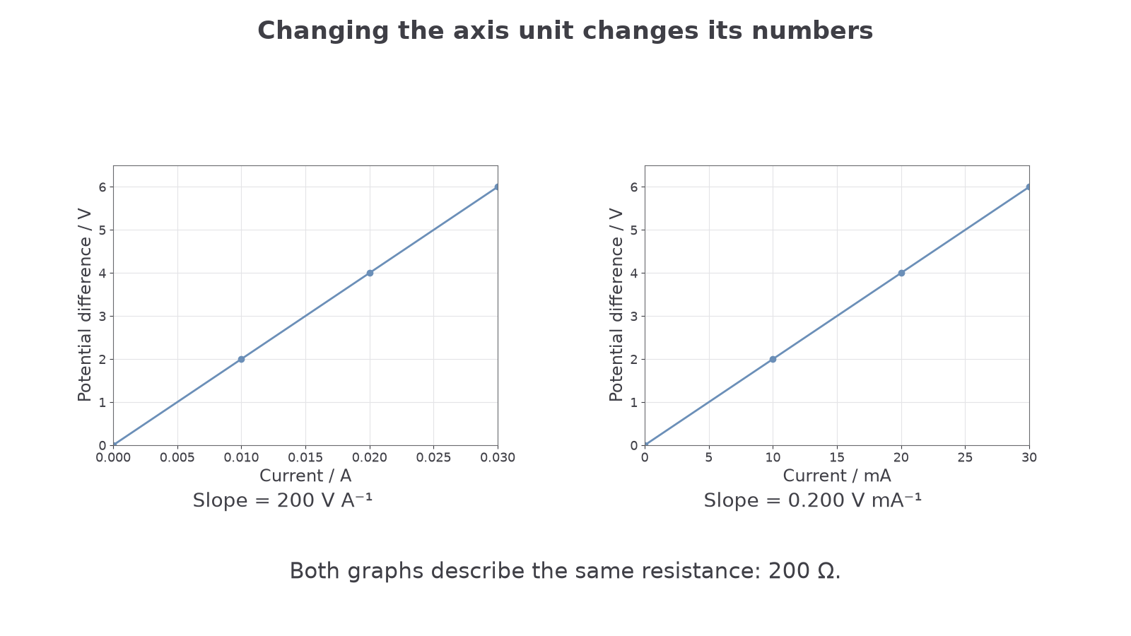
This means the numbers written in the column or read from the axis are numerical values in that unit. If the axis says $\text{current} /\mathrm{mA}$, a plotted value of 12 means $12\ \text{mA}$, which is $12 \times 10^{-3}\ \text{A}$.

Tables follow the same idea. Put the unit in the heading, not repeatedly in the body:

Do not write units after every number inside the data cells. That makes data harder to scan and is not good practical style.

For graph axes, a scale factor can also be included in the label. For example:

$1/R / 10^{-6} \Omega^{-1}$

means that the plotted number is the value of $1/R$ divided by $10^{-6}\ \Omega^{-1}$. A plotted value of 4.0 corresponds to:

This convention lets very small or very large values fit neatly onto a graph. It is still your responsibility to carry the scale factor into any calculation involving the gradient, intercept or read-off.

Logarithms are a special case. You can only take the logarithm of a quantity with no units, such as a ratio. A graph label such as $\ln(V / V_0)$ is acceptable because $V/V_0$ is dimensionless.

Worked example: correcting labels

A student records a table with headings:

A better table is:

The improved version states the physical quantity, separates the unit using a solidus, and keeps units out of the body of the table.
[DIAGRAM: asset_slug: units_graph_scale; caption: Current axes in amperes and milliamperes give different numerical gradients but the same resistance of 200 Ω.; description: The same current data shown in amperes and milliamperes: axis scaling changes the numerical slope, while the resistance remains 200 Ω.]