6.3.3(f) - Transformers

The transformer model

A simple transformer has two coils wound on the same laminated iron core. The coil connected to the input supply is the primary coil. The coil connected to the output circuit is the secondary coil.

The primary supply must be alternating for continuous operation. An alternating current in the primary coil produces an alternating magnetic flux in the iron core. This changing flux links the secondary coil and induces an alternating e.m.f. across the secondary.

The detailed Faraday-law equation belongs with the induction lesson. The transformer link you need here is simple: no changing magnetic flux means no continuous induced e.m.f. in the secondary. A steady d.c. supply may give a momentary effect when switched on or off, but it is not suitable for a normal transformer and can overheat the primary coil.

[DIAGRAM: asset_name: 6.3.3(f) - Transformers - diagram 1; asset_slug: 6_03_3b_transformers_and_induction_applications__diagram_01; recommended_method: drawn_physics; caption: A transformer transfers energy between separate primary and secondary circuits through a magnetic core.; description: Connected primary and secondary coil symbols with separate circuits and laminated magnetic core.]

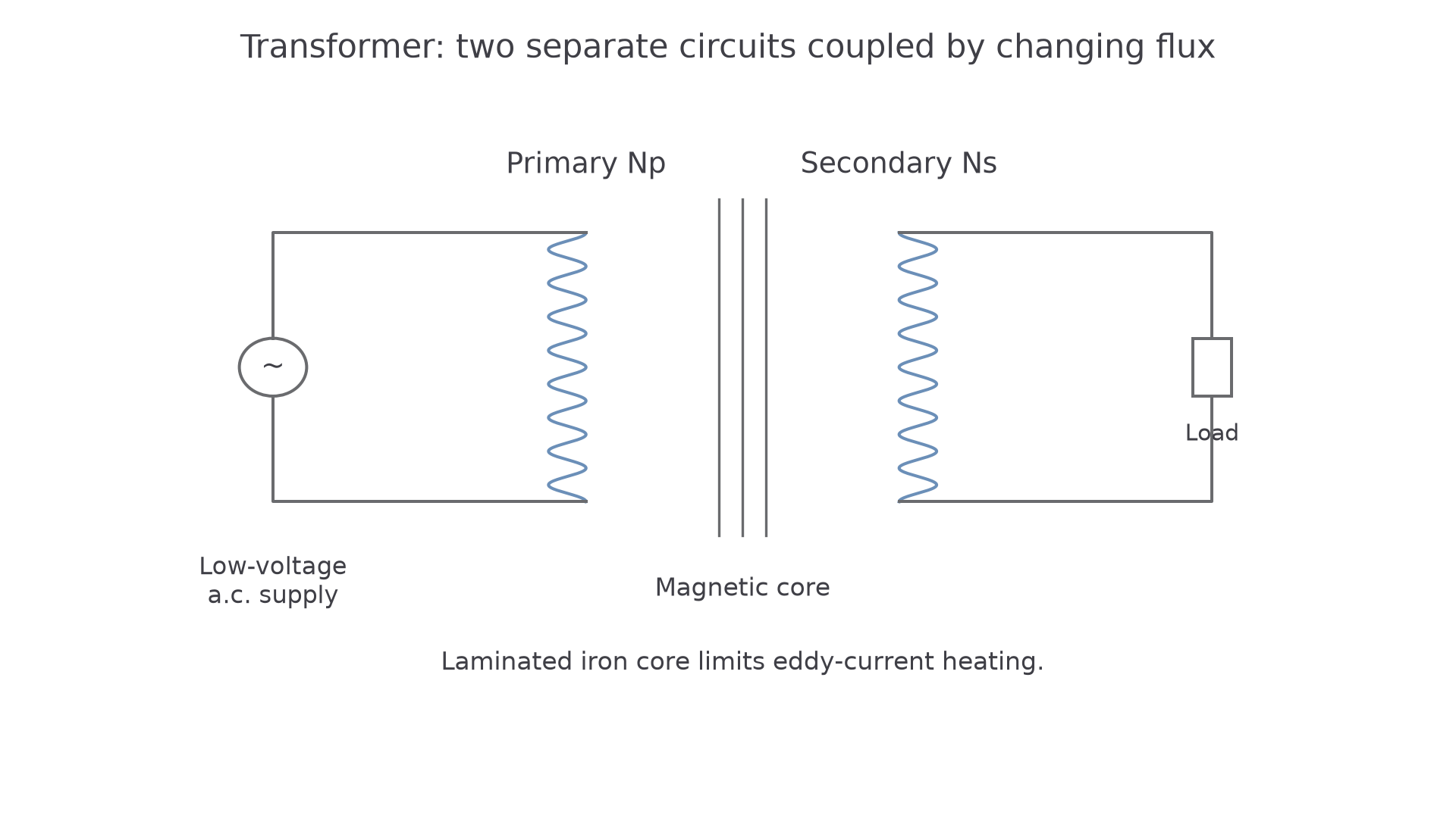
The iron core has a high permeability, so it provides an easy magnetic path for the changing flux. That means a large fraction of the changing flux produced by the primary links the secondary.

The core is laminated: it is made from thin insulated sheets rather than one solid block. A changing magnetic field can induce currents in a conducting core. These eddy currents cause heating and waste energy. Laminating the core makes the current paths much smaller, so eddy current losses are reduced.

Two transformer words are useful from the start:

• a step-up transformer has more secondary turns than primary turns, so it gives a larger secondary p.d.
• a step-down transformer has fewer secondary turns than primary turns, so it gives a smaller secondary p.d.

Ideal transformer ratios

OCR gives the ideal-transformer relationship in terms of turns, p.d. and current:

Here $N_p$ and $N_s$ are the numbers of turns on the primary and secondary coils. $V_p$ and $V_s$ are the primary and secondary p.d.s. $I_p$ and $I_s$ are the primary and secondary currents. In transformer work these p.d.s and currents are usually a.c. meter readings, so treat them as rms values unless a question states otherwise.

The first equality gives the voltage ratio:

So if the secondary has twice as many turns as the primary, the secondary p.d. is twice the primary p.d. If the secondary has one tenth as many turns, the secondary p.d. is one tenth of the primary p.d.

The current ratio is inverse:

This is the part students most often say backwards. In an ideal step-up transformer, $V_s$ is larger but $I_s$ is smaller. In an ideal step-down transformer, $V_s$ is smaller but $I_s$ is larger.

Worked example: a step-down transformer

A transformer has $500$ turns on the primary coil and $50$ turns on the secondary coil. The primary p.d. is $12.0\ \mathrm{V}$. The primary current is $0.20\ \mathrm{A}$. Assume the transformer is ideal.

First find the secondary p.d.:

Now use the inverse current ratio:

The transformer has stepped the p.d. down by a factor of $10$, so the ideal secondary current is $10$ times the primary current.

Power and applications

The ideal-transformer equation contains the current ratio because an ideal transformer conserves power. There is no energy loss in the ideal model, so:

This is not a separate new rule to memorise; it is another way of saying that energy is transferred from the primary circuit to the secondary circuit without loss in the ideal model.

In a real transformer, the output power is slightly less than the input power. Energy can be lost by heating in the coil resistance, eddy currents in the core, imperfect flux linkage, and repeated magnetisation of the core. For this lesson, the essential OCR point is that the laminated iron core reduces eddy-current heating, and the ideal equations assume these losses are negligible.

Transformers are useful because many applications need a particular voltage-current combination. For transmission of electrical power, stepping up the p.d. makes the current smaller for the same power:

If $P$ is fixed and $V$ is increased, $I$ must decrease. Heating loss in cables depends on current:

So a high transmission voltage gives a lower current and much lower heating loss in the cables. A step-down transformer can then reduce the p.d. near the user to a safer and more useful value.

Worked example: current in transmission cables

A transformer supplies $2.0\ \mathrm{MW}$ of power to transmission cables.

At $20\ \mathrm{kV}$:

At $200\ \mathrm{kV}$: