4.3.2 - Internal resistance

E.m.f., Terminal P.d. and Lost Volts

A source of e.m.f. is a device such as a chemical cell or power supply that transfers energy to charges. A real source also has some resistance inside it, so some energy is transferred inside the source whenever current flows.

This definition is about energy, not force. In a cell, chemical energy is transferred to electrical energy carried by the moving charge. In a power supply, energy may come from an external electrical source.

The terminal p.d. is the p.d. across the terminals of the source. In a simple circuit with one external load resistor, it is also the p.d. across that load resistor. When current flows, the terminal p.d. is less than the e.m.f. because some energy per coulomb is transferred inside the source.

The phrase "lost volts" is slightly misleading. The energy is not destroyed; it is transferred inside the source, usually as thermal energy. Increasing the current increases $Ir$, so it reduces the terminal p.d. available to the external circuit.

Worked example: energy per unit charge in a working cell

A cell has e.m.f. $1.50\,\mathrm{V}$. When it supplies a current of $0.400\,\mathrm{A}$, the terminal p.d. is $1.26\,\mathrm{V}$.

The lost volts are:

The internal resistance is:

So each coulomb receives $1.50\,\mathrm{J}$ from the cell, $1.26\,\mathrm{J}$ is transferred in the external circuit, and $0.24\,\mathrm{J}$ is transferred inside the cell.

Sources with the same open-circuit e.m.f. can perform differently under load. At $0.50\,\mathrm A$, a $1.50\,\mathrm V$ cell with $r=0.20\,\Omega$ gives $1.40\,\mathrm V$, while one with $r=1.0\,\Omega$ gives only $1.00\,\mathrm V$. A device requiring at least $1.20\,\mathrm V$ at that current would work with the first but not the second under these conditions. Selecting a source therefore involves its loaded performance, current rating and heating, as well as price, capacity and replacement or disposal costs. The open-circuit voltage alone does not establish suitability.

The Source Model and OCR Equations

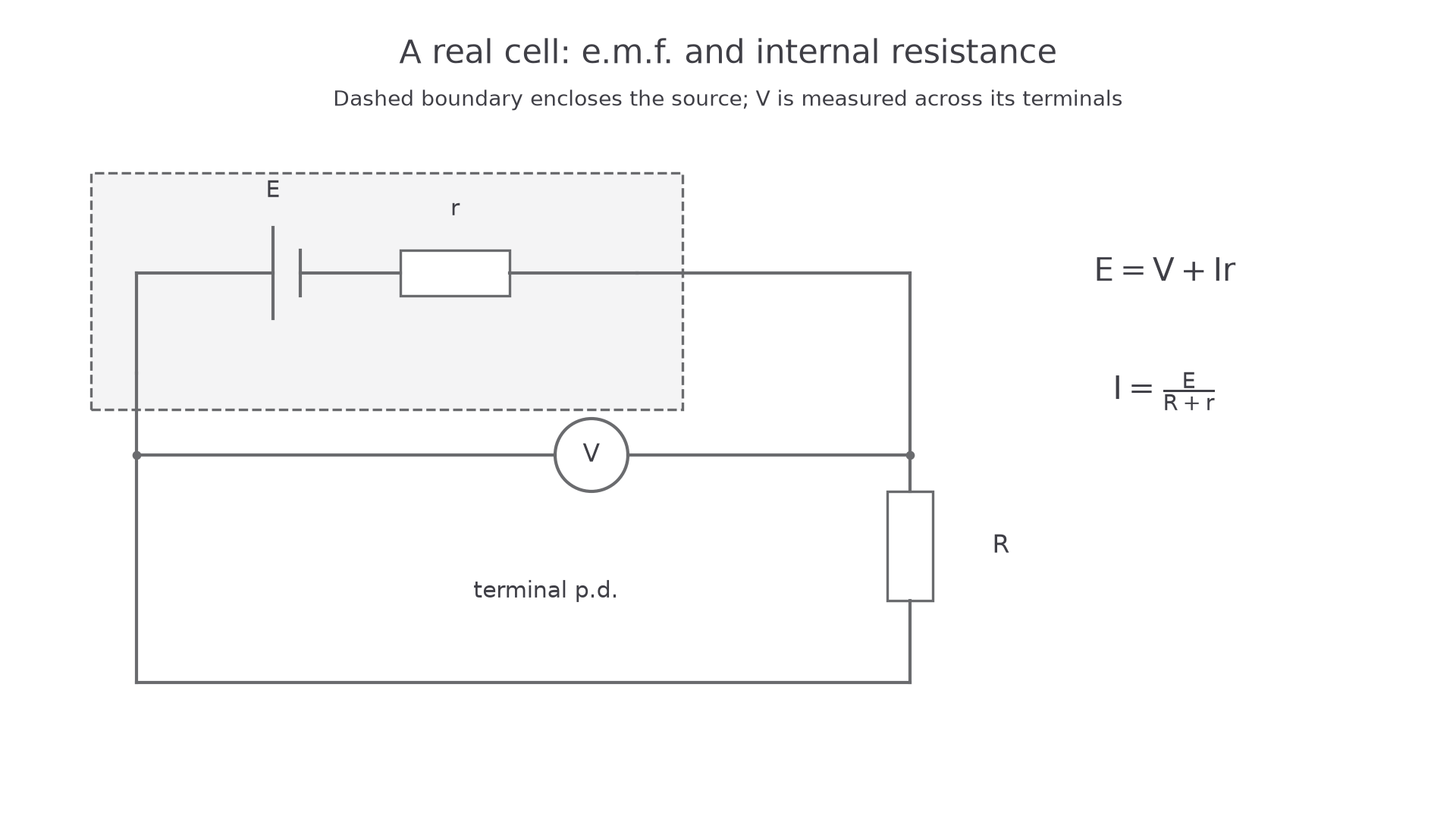
The useful model is an ideal source of e.m.f. $E$ in series with an internal resistance $r$. The external circuit is represented by a load resistance $R$. The same current $I$ passes through $R$ and $r$ because they are in series.

The energy balance per coulomb is:

Here:

• $E$ is the e.m.f. of the source in V.
• $V$ is the terminal p.d. in V.
• $I$ is the current in A.
• $r$ is the internal resistance in $\Omega$.
• $Ir$ is the lost volts in V.

If the external circuit is a single load resistor $R$, then $V = IR$, so:

This is just Kirchhoff's second law applied to the complete loop: the energy per coulomb supplied by the source equals the energy per coulomb transferred across the external resistance plus the energy per coulomb transferred across the internal resistance.

Two limiting cases are worth keeping straight:

• Open circuit: $I = 0$, so $Ir = 0$ and the terminal p.d. is equal to the e.m.f.
• Large current: $Ir$ is larger, so the terminal p.d. is smaller.

Do not treat the internal resistance as a separate visible component you can disconnect from the cell. It is a model for the energy transfers inside the source.

[DIAGRAM: asset_slug: 4_03_2_internal_resistance__diagram_01; description: A real source is modelled as an ideal source in series with internal resistance.; caption: An ideal source and internal resistance model a real cell.]

Rearranging for Graphs

OCR questions often test whether you can choose a straight-line graph from the internal-resistance equation. Start from the equation, then compare it with the form:

For a direct terminal p.d. method:

Rearrange to:

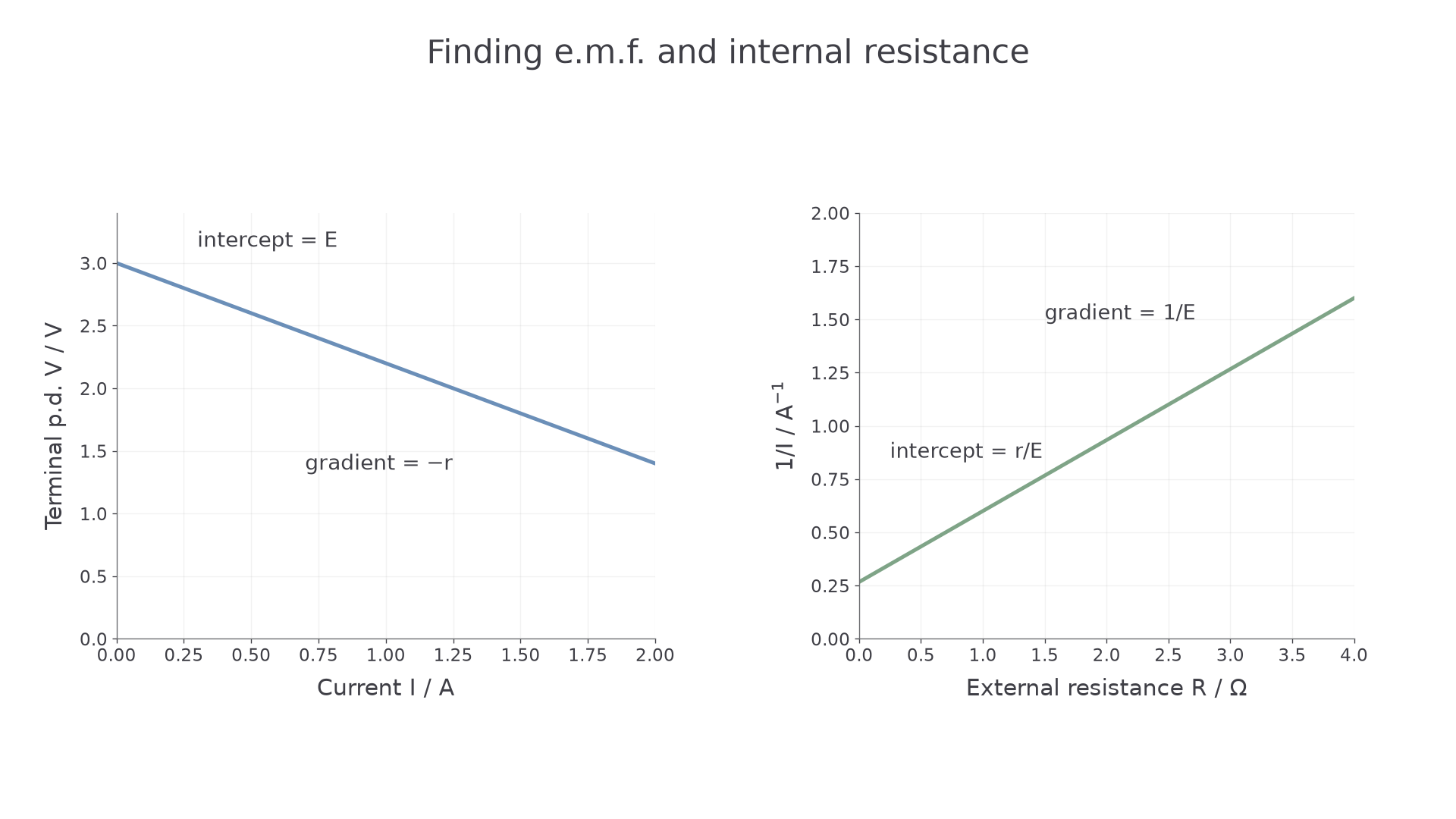
If you plot terminal p.d. $V$ on the vertical axis against current $I$ on the horizontal axis:

• the vertical intercept is $E$
• the gradient is $-r$
• the magnitude of the gradient is the internal resistance

For a method where the external resistance $R$ is varied and current is measured, use:

Divide both sides by $EI$:

If you plot $1/I$ against $R$:

• the gradient is $1/E$
• the vertical intercept is $r/E$
• if $E$ is known, $r = E \times \text{intercept}$
• if $E$ is not known, $r = \text{intercept} / \text{gradient}$

Worked example: using an intercept from $1/I$ against $R$

A student plots $1/I$ against $R$ for a cell of e.m.f. $5.0\,\mathrm{V}$. The vertical intercept is $0.20\ \mathrm{A}^{-1}$.

From the rearranged equation:

So:

The unit works because $\mathrm{V}\,\mathrm{A}^{-1}$ is an ohm.

[DIAGRAM: asset_slug: 4_03_2_internal_resistance__diagram_02; description: Two straight-line methods give the e.m.f. and internal resistance from intercepts and gradients.; caption: Two graph methods for finding e.m.f. and internal resistance.]