4.2.4 - Resistivity and temperature dependence

Resistivity as a material property

The resistance of a uniform wire depends on three things: the material, the length of the conducting path, and the cross-sectional area available for charge flow. Resistivity is the material part of that story.

In this equation, $R$ is resistance in ohms $(\Omega)$, $\rho$ is resistivity in ohm metres $(\Omega\,\mathrm{m})$, $L$ is length in metres, and $A$ is cross-sectional area in square metres. Rearranging gives:

The units come from the rearranged equation:

That unit is often where mistakes start. Resistivity is not measured in $\Omega\,\mathrm{m^{-1}}$. The factor $A/L$ turns the resistance of a particular sample into a material property.

The shape dependence is physical. A longer wire gives charge carriers more material to pass through, so resistance is larger. A larger cross-sectional area gives more parallel paths through the material, so resistance is smaller. For the same material and temperature:

• doubling $L$ doubles $R$
• doubling $A$ halves $R$
• changing the material changes $\rho$

Worked example: resistance of a metal wire

A uniform wire has resistivity $1.1 \times 10^{-6}\ \Omega\,\mathrm{m}$, length $1.50\ \mathrm{m}$, and diameter $0.35\ \mathrm{mm}$. Find its resistance.

First convert the diameter:

For a circular cross-section:

Now substitute into $R = \rho L/A$:

To two significant figures, $R = 17\ \Omega$.

Using a graph to find resistivity

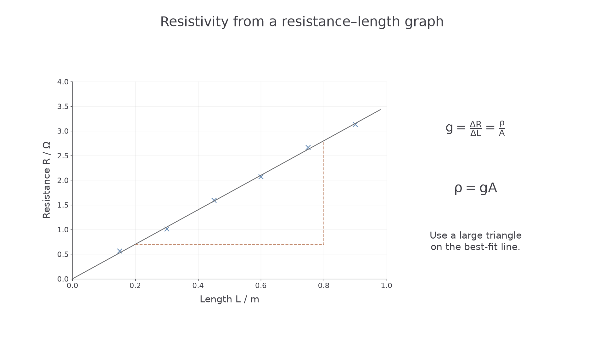
For one wire of fixed material and fixed diameter, $\rho$ and $A$ are constant. The equation

has the same form as $y = mx$ if you plot $R$ on the vertical axis and $L$ on the horizontal axis:

So:

The graph method is usually better than using just one length because it uses all the readings and makes anomalies easier to spot. A good line of best fit should be thin and clear. Do not join point-to-point unless the data actually justify a non-linear curve; for a uniform metal wire at constant temperature, the expected relationship between $R$ and $L$ is linear.

Worked example: graph gradient

A metal wire has diameter $0.40\ \mathrm{mm}$. A graph of resistance $R$ against length $L$ gives a best-fit gradient of $8.6\ \Omega\,\mathrm{m}^{-1}$. Calculate the resistivity of the wire.

Convert diameter:

Calculate area:

Use $\rho = \text{gradient} \times A$:

To two significant figures, $\rho = 1.1 \times 10^{-6}\ \Omega\,\mathrm{m}$.

A constant extra lead or contact resistance gives $R_{\rm measured}=\rho L/A+R_0$. The intercept is then $R_0$; the gradient can still estimate $\rho/A$. Do not force the fitted line through the origin when the data support a non-zero intercept. A contact resistance that changes between readings instead causes scatter or bias and is not removed by simply fitting a line.

To estimate gradient uncertainty, plot error bars from the measurement limits and draw the steepest and shallowest straight lines consistent with those bars. If the best gradient is $8.6\,\Omega\,\mathrm{m^{-1}}$ and acceptable gradients span $8.2$ to $9.0\,\Omega\,\mathrm{m^{-1}}$, an appropriate symmetric estimate is $8.6\pm0.4\,\Omega\,\mathrm{m^{-1}}$, or about $4.7\%$. A diameter uncertainty of $2.0\%$ contributes $4.0\%$ to area, so the conservative resistivity uncertainty is about $8.7\%$. A visually steep or shallow line that misses the error bars is not an acceptable limiting fit.

[DIAGRAM: asset_slug: 4_02_4_resistivity_and_temperature_dependence__diagram_02; description: The gradient of a resistance–length graph is resistivity divided by cross-sectional area.; caption: The gradient of a resistance–length graph gives resistivity divided by area.]

PAG3 metal-wire resistivity method

The practical aim is to determine the resistivity of a metal. To do that, you need measurements of resistance, length and cross-sectional area. A typical method uses a long uniform resistance wire taped beside a metre rule, with a movable contact to vary the length of wire in the circuit.

A strong written method includes these steps.

1. Measure the diameter of the wire using a micrometer or suitable calipers at several positions and in different orientations. Calculate the mean diameter.
2. Calculate the cross-sectional area using $A = \pi d^2/4$.
3. Connect the test length of wire in a low-voltage DC circuit with an ammeter in series.
4. Connect the voltmeter in parallel across the measured length of wire, not across the whole supply.
5. Use a fixed contact at one end and a movable contact or flying lead to set different lengths $L$.
6. For each length, record the p.d. $V$ and current $I$, then calculate $R = V/I$.
7. Repeat readings where sensible, switch off between readings, and plot $R$ against $L$.
8. Find the gradient of the best-fit line and calculate $\rho = \text{gradient} \times A$.

Heating matters because the resistivity of a metal changes with temperature. If the wire warms as current passes through it, the resistance can change for a reason other than length. Use a small current, switch off between readings, and avoid leaving the flying lead on one point for a long time.

Uncertainty reasoning should be specific.