S6 - Scatter graphs and correlation

Plotting paired numerical data

Can a shallow scatter-graph trend be stronger than a steep one? Yes: steepness describes a rate, while strength describes how closely points follow a pattern. We will separate those ideas before trusting any prediction.

A teacher records practice time and quiz score for each pupil. The two measurements from one pupil must stay paired. Sorting each column separately would invent relationships that were never observed.

Plot small crosses or clear points. Do not join successive points: these are different pupils, not one quantity changing through time. Two pupils may share the same practice time but have different scores, so two points can lie above the same horizontal position.

Change only the pupil selected from the table. The axis roles stay fixed.

[DIAGRAM: asset_name: Practice time and quiz scores; asset_slug: aqa8300_s05_scatter; caption: Each cross represents one pupil's paired measurements, without joining the crosses; description: A scatter graph with practice time from 0 to 70 minutes horizontally and score from 0 to 20 vertically plots 10,3 then 20,7 then 30,8 then 40,12 then 50,13 then 60,17. The points 20,7 and 40,12 are labelled.]

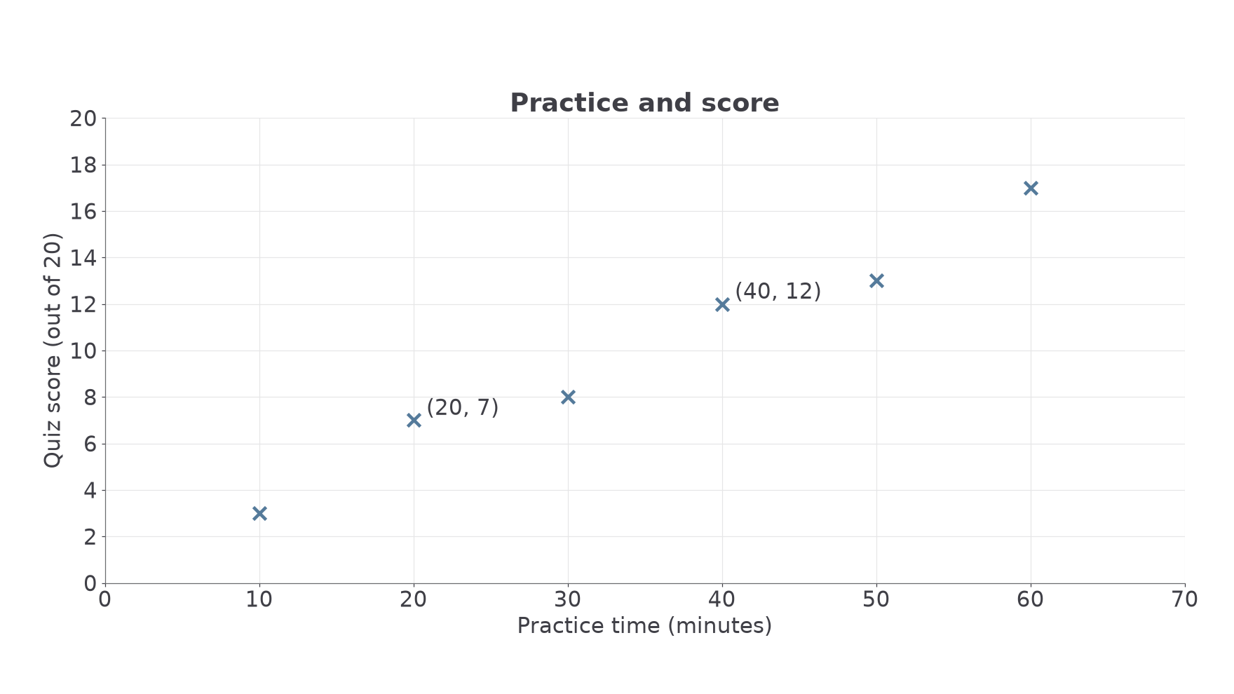
These plotting conventions are not on the formulae sheet: learn them.

The next two pairs belong to two different cyclists.

Direction and strength of correlation

Read a scatter graph from left to right. If larger $x$-values tend to go with larger $y$-values, the association is positive. If they tend to go with smaller $y$-values, it is negative. A tendency allows exceptions; it does not require every point to rise or fall in order.

Use both direction and strength when requested: “strong positive correlation”, for example. “Going up” describes an impression but does not give the statistical term. A single unusual point may be an outlier; it does not automatically cancel the pattern among the others.

[DIAGRAM: asset_name: Types and strengths of correlation; asset_slug: aqa8300_s05_correlation; caption: Direction and closeness to a trend are separate features; description: Four labelled scatter panels show strong positive correlation, weak positive correlation, strong negative correlation and no correlation. Identical axis ranges make direction easy to compare, but the captions emphasise spread around the trend rather than steepness.]

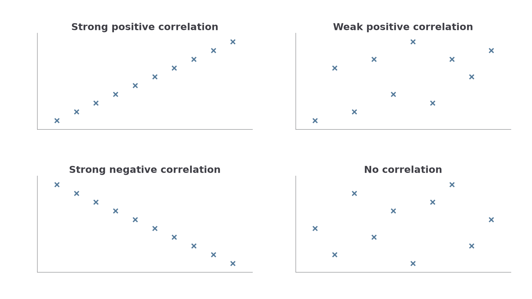
Here is a useful surprise: converting practice time from minutes to seconds makes every horizontal number $60$ times larger and the numerical gradient $60$ times smaller. It does not weaken the relationship between the pupils' measurements. Points exactly on a rising straight line show perfect positive correlation whether that line is shallow or steep.

These terms are not on the formulae sheet: learn them. With no useful trend, a straight-line prediction has little support; do not draw a line simply because a question contains a scatter graph.

Drawing an estimated line of best fit

An estimated line of best fit summarises a roughly straight trend. Draw one straight line through the middle of the point cloud, following its direction, with points reasonably balanced above and below across the range.

It need not pass through a particular data point or the origin. Two extreme observations do not automatically fix it. Do not join the crosses with a zigzag. Use the overall pattern and a ruler; small differences between sensible estimated lines are expected.

The line drawn below for the practice data has equation $y=0.25x+1.5$. An equation is useful here because earlier work on straight lines lets us check readings; drawing an estimated line does not require calculating an exact regression formula.

Change only one observation by adding a pupil at $(35,19)$. That point lies well away from the existing pattern.