S3 - Histograms (Higher)
Construct and interpret histograms for continuous and grouped discrete data, including unequal class widths. Use frequency density to make area represent frequency, recover a missing scale, and estimate counts within a class while stating the assumption.
Frequency is area (Higher)
One histogram bar is units wide and units high. Another is units wide and units high. Which represents more observations? The taller bar loses: its area is , while the shorter bar's area is . A histogram asks you to look at area, not height alone.
You already know
A grouped frequency table hides individual observations inside intervals. Midpoints can estimate a mean, but the class width is the upper boundary minus the lower boundary.
Suppose observations are spread across a width of . There are observations per unit of width. Across a width of , the same frequency would give only per unit. That “per unit” height is frequency density.
Histogram and frequency density
A histogram represents grouped numerical data with touching bars whose widths match the class intervals. Bar area is proportional to frequency. Frequency density is frequency divided by class width. Unlike a categorical bar chart, the horizontal axis is a continuous numerical scale, and a wide class must occupy more space.
The vertical scale makes the rectangle's area give the class frequency directly.
Frequency density
For a class , its width is , not its midpoint. Use the same horizontal units throughout.
Not on the formulae sheet: learn it.
Label both axes and choose a convenient regular vertical scale before drawing bars.
Worked example 1: equal class widths
Question. Time classes , , have frequencies . Work out frequency densities and draw the histogram. Non-calculator.
Plan. Divide each frequency by its width , then draw touching rectangles.
Why this step? Equal widths make heights proportional to frequencies, but using density still gives the correct area rule.
Answer. Draw bars over to , to , to , with heights . Label the vertical axis “Frequency density”.
Check. Areas are , , , matching the table.
Change only the last upper boundary from to . Its frequency stays , so its height must fall.
Worked example 2: one wider class
Question. Classes , , have the same frequencies . Draw the new histogram. Non-calculator.
Plan. Keep the first two densities, but divide the last frequency by the new width .
Why this step? A bar twice as wide needs half the height to keep its frequency, and therefore its area, unchanged.
Answer. Draw touching bars with heights over the three stated intervals.
Check. The last area is , just as before.
[DIAGRAM: asset_name: Equal and unequal histogram widths; asset_slug: aqa8300_s06_construct; caption: Doubling the last class width halves its density while keeping frequency 15; description: Two frequency-density histograms show the two worked tables on identical time and density scales. Left widths 5,5,5 and heights 2,4,3. Right widths 5,5,10 and heights 2,4,1.5. The last bars are labelled frequency 15.]
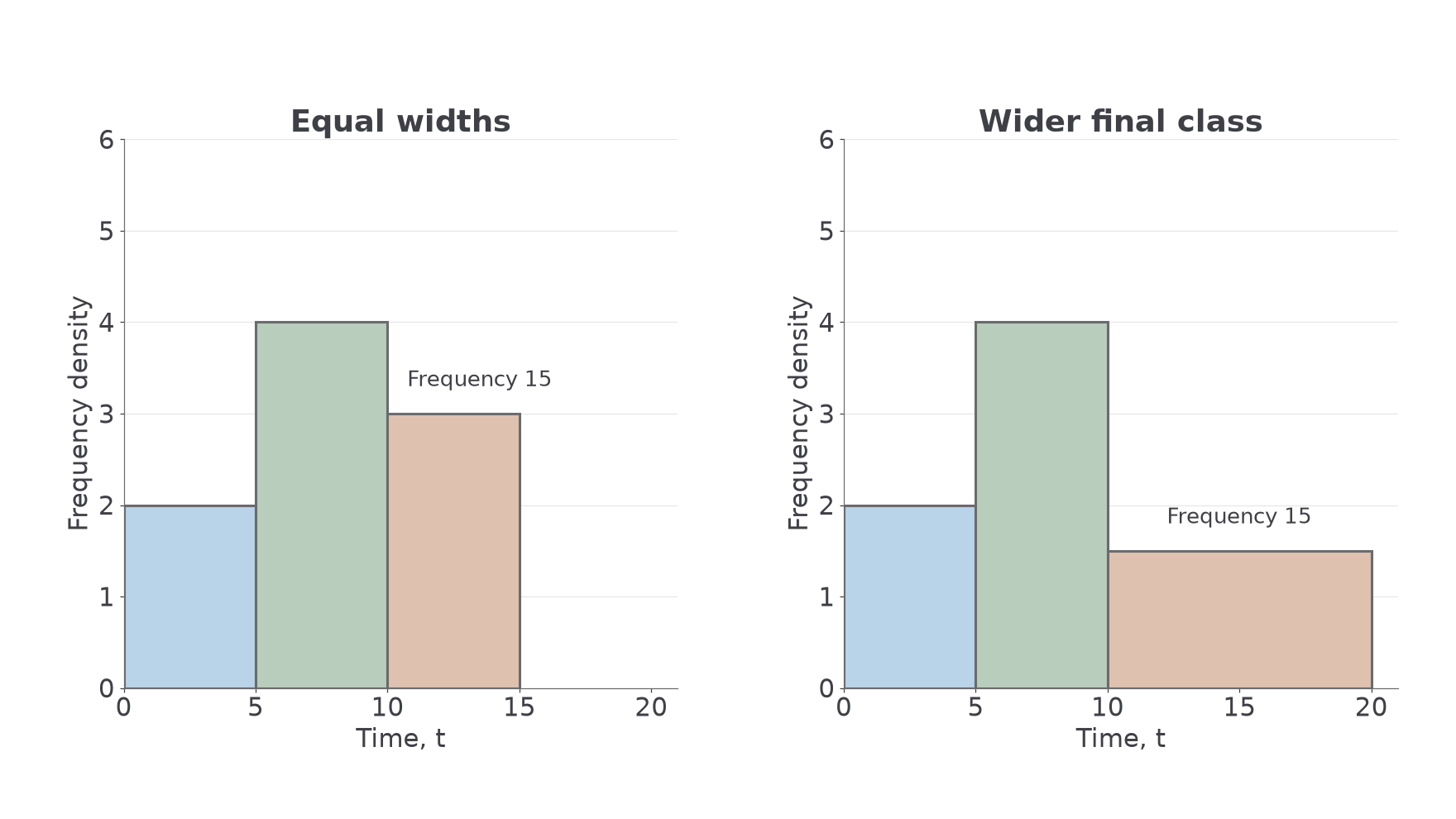
The bar's horizontal boundaries and vertical height must both be correct.
Watch out
Wrong: draw heights with unequal widths. The last bar then has too much area. Right: use frequency density, not frequency, for its height.
Work out the heights before reaching for a ruler.
Reading frequencies and a missing scale (Higher)
Reading a histogram reverses its construction: multiply width by density. If the density scale is missing, a known bar can establish how drawing area relates to frequency.
For example, a bar with frequency and width must have density , whatever physical height appears on the page. Use that known height to calibrate the vertical scale, then read the other heights consistently.
Worked example 3: a labelled density axis
Question. A bar covers and has frequency density . Work out its frequency. Non-calculator.
Plan. Multiply the interval width by its height on the density scale.
Why this step? Density counts observations per unit of width, so multiply by the number of width units.
Answer. observations.
Check. , recovering the density.
Change only the available scale: the axis now has no density numbers, but one frequency is known.
Worked example 4: using a known bar
Question. On a histogram grid, a reference bar is horizontal units wide and grid units high. It represents observations. Another bar is units wide and grid units high. Work out its frequency. Non-calculator.
Plan. Find observations per unit of drawn area from the reference bar.
Why this step? With an unlabelled vertical scale, a numerical grid height need not already be the frequency density. The known bar tells you the conversion.
Answer. observations, so the shorter bar represents more than the reference bar.
Check. Its area is times the reference area; .
[DIAGRAM: asset_name: Calibrating an unlabelled histogram; asset_slug: aqa8300_s06_scale; caption: A known bar sets the area-to-frequency scale before another bar is read; description: Touching rectangles have horizontal widths 5 and 10 and drawn heights 4 and 3. Horizontal grid lines are visible but vertical tick labels are absent. The first bar is labelled frequency 20 and the second frequency unknown. Brackets state the widths and the grid heights.]
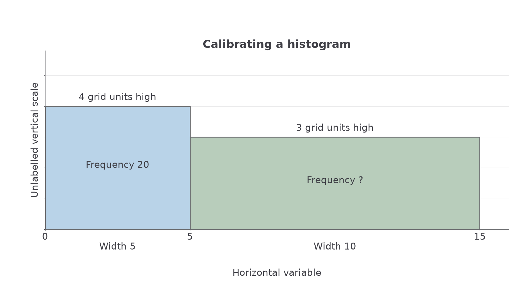
Use areas in consistent drawing units. Mixing centimetres for one bar with squares for another destroys the comparison.
Watch out
Wrong: compare only the heights and , then conclude the second frequency is smaller. Right: compare areas and , because the widths differ.
The scale factor in the next diagram description is not .
Continue this lesson.
You’re previewing NovaLearn without an account. Create a free account to read the rest.
Create free account