S3, S4 - Cumulative frequency and box plots (Higher) | AQA GCSE Mathematics

Construct cumulative frequency graphs, estimate medians and quartiles, and use five-number summaries to draw box plots. Compare distributions using medians and interquartile ranges, and distinguish what these displays reveal from what they hide.

Building a cumulative frequency graph (Higher)

One section of a box plot is much longer than another. Does that mean it contains more observations? The surprising answer is that long and short sections can each represent roughly a quarter of the data. To see why, start with a graph that counts observations up to each boundary.

You already know

A grouped table gives frequencies in intervals. Adding frequencies gives a total, but individual measurements remain hidden. A graph reading from grouped data is an estimate.

For frequencies $10,20,20,10$ , the running totals are $10,30,50,60$ . After the second class, $30$ observations have been counted altogether, not just the $20$ in that class.

Cumulative frequency

The number of observations up to a given boundary, found by adding the frequencies of all classes up to that point. For classes ending with $t\leqslant b$ , plot the cumulative frequency at $b$ , the upper class boundary. Include zero at the lowest boundary before any observations have been counted.

Plot measurement horizontally and cumulative frequency vertically. Label units and use regular scales. Join the points in order with straight segments or a smooth increasing curve; do not force the graph through a point it should miss. The graph cannot decrease because adding another class cannot remove observations. A zero-frequency interval gives a horizontal section.

Worked example 1: running totals at upper boundaries

Question. Classes $0<t\leqslant10$ , $10<t\leqslant20$ , $20<t\leqslant30$ , $30<t\leqslant40$ , in minutes, have frequencies $10,20,20,10$ . Draw a cumulative frequency graph. Non-calculator.

Plan. Add frequencies successively and plot each total at its upper boundary.

\begin{aligned} \text{cumulative frequencies}&=10,\ 10+20,\ 30+20,\ 50+10 &&\text{running totals}\\ &=10,30,50,60 &&\text{evaluate}\\ \text{plot}&:(0,0),(10,10),(20,30),(30,50),(40,60) &&\text{include the start} \end{aligned}

Why this step? By the time the boundary $20$ is reached, both first classes have been included. A class midpoint would place their total too early.

Answer. Plot the five points and join them with an increasing graph. The first panel below uses straight segments.

Check. The final height $60$ equals the total frequency, and successive rises are $10,20,20,10$ .

Change only the last frequency from $10$ to $20$ . The first three running totals stay fixed.

Worked example 2: a larger final class

Question. The same classes now have frequencies $10,20,20,20$ . Draw the new cumulative frequency graph. Non-calculator.

Plan. Keep the first three cumulative frequencies and update the final total.

\begin{aligned} \text{cumulative frequencies}&=10,30,50,70 &&\text{last total gains ten}\\ \text{plot}&:(0,0),(10,10),(20,30),(30,50),(40,70) &&\text{upper boundaries} \end{aligned}

Why this step? Changing the last class cannot change how many measurements were already counted at earlier boundaries.

Answer. Use the second panel below: the final point is now $(40,70)$ .

Check. The rise from $30$ to $40$ is $20$ , matching the new last frequency.

[DIAGRAM: asset_name: Constructing cumulative frequency graphs; asset_slug: aqa8300_s07_construct; caption: Running totals are plotted at upper boundaries, with zero at the starting boundary; description: Two labelled cumulative frequency graphs use the same axes. Left joins 0,0 then 10,10 then 20,30 then 30,50 then 40,60. Right has the same first four points but ends 40,70. All points are marked and joined by straight segments.]
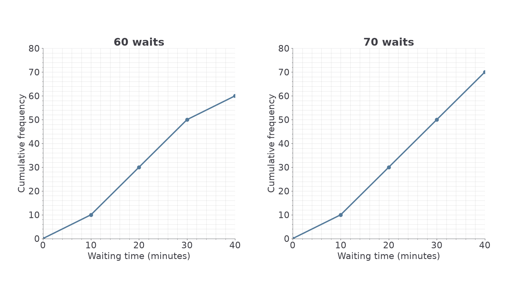
Running totals are plotted at upper boundaries, with zero at the starting boundary

These plotting conventions are not on the formulae sheet: learn them. A cumulative graph is useful for questions about values below a threshold or the value reached by a given fraction of the data.

Watch out

Wrong: plot each ordinary frequency at its class midpoint. That does not create cumulative frequency. Right: use running totals at upper boundaries.

Work out a fresh set of running totals and the coordinates they belong to.

Median, quartiles and interquartile range (Higher)

The median splits ordered data into halves. Quartiles locate the halfway points of those halves, separating approximately four quarters. Ties can make the split less visually obvious, but the idea is still about positions, not equal distances along the scale.

Quartiles and interquartile range

The lower quartile $Q_1$ is the value about a quarter of the way through ordered data. The upper quartile $Q_3$ is about three quarters of the way through. The interquartile range, $\mathrm{IQR}=Q_3-Q_1$ , measures the spread of the middle half of the data.

For a short ordered list, use the median of the lower half and the median of the upper half; when there is one middle observation, leave it out of both halves. For example, $2,4,6,8,10,12,14,16$ has median $9$ , lower-half median $5$ , upper-half median $13$ , and IQR $8$ .

For a grouped cumulative graph, use fractions of the total frequency instead. Read horizontally from a cumulative-frequency level to the graph, then vertically down to the measurement axis.

Quartile levels on a cumulative frequency graph

For total frequency $N$ , read:

\begin{aligned} Q_1&\text{ at cumulative frequency }N/4\\ \text{median}&\text{ at cumulative frequency }N/2\\ Q_3&\text{ at cumulative frequency }3N/4\\ \mathrm{IQR}&=Q_3-Q_1 \end{aligned}

The graph readings estimate measurement values. The cumulative-frequency levels themselves are not the quartiles.

Not on the formulae sheet: learn it.

The next readings use the straight-segment graphs from Part 1. A smooth curve may give slightly different estimates; use your own drawn graph consistently.

Worked example 3: reading three fractional positions

Question. Use the cumulative graph for $60$ waits to estimate the median, quartiles and IQR. Non-calculator.

Plan. Mark levels $15,30,45$ , then read the corresponding times.

\begin{aligned} N/4&=60/4=15 &&\text{lower-quartile level}\\ N/2&=30,\qquad3N/4=45 &&\text{middle and upper levels}\\ Q_1&\approx12.5,\quad\text{median}\approx20,\quad Q_3\approx27.5 &&\text{read across, then down}\\ \mathrm{IQR}&\approx27.5-12.5=15 &&\text{subtract the time readings} \end{aligned}

Why this step? The vertical coordinate counts waits; the horizontal coordinate is the waiting time requested.

Answer. Estimated $Q_1=12.5$ minutes, median $20$ minutes, $Q_3=27.5$ minutes, IQR $15$ minutes.

Check. The middle half stretches from about $12.5$ to $27.5$ , with the median between them.

Change only the total and final class to use the second graph. The quartile levels must change too.

Worked example 4: a different total frequency

Question. Use the cumulative graph for $70$ waits to estimate the same measures. Calculator allowed.

Plan. Recalculate the fractional levels before reading this graph.

\begin{aligned} N/4&=17.5,\qquad N/2=35,\qquad3N/4=52.5 &&\text{fractions of 70}\\ Q_1&\approx13.75,\quad\text{median}\approx22.5,\quad Q_3\approx31.25 &&\text{straight-segment readings}\\ \mathrm{IQR}&\approx31.25-13.75=17.5 &&\text{difference of quartiles} \end{aligned}

Why this step? Reusing the old levels $15,30,45$ would locate the wrong fractions of the new sample.

Answer. Approximately $13.8$ , $22.5$ , $31.3$ minutes for the three quartiles, and $17.5$ minutes for IQR.

Check. More long waits raise the median from $20$ to $22.5$ . Use unrounded readings for the IQR.

[DIAGRAM: asset_name: Quartile readings from cumulative frequency; asset_slug: aqa8300_s07_quartiles; caption: The three levels are fractions of the total frequency, while the answers are read on the time axis; description: The 60-wait cumulative graph has dashed horizontal guides at 15,30,45 and vertical guides to 12.5,20,27.5 minutes. The three time readings are labelled below the graph.]
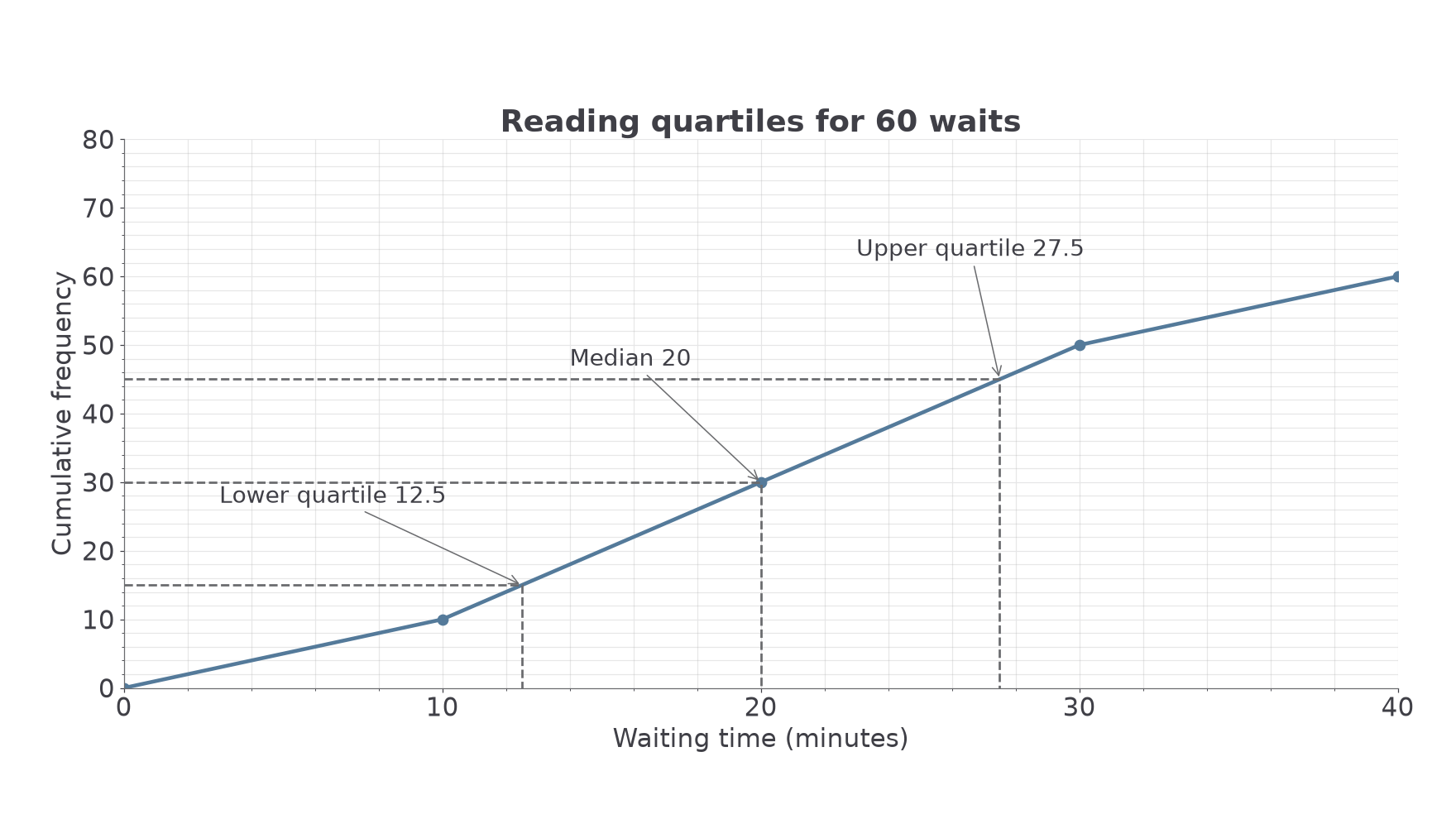
$The three levels are fractions of the total frequency, while the answers are read on the time axis$

A count below a threshold is read in the other direction: go up from the time to the graph, then across to the cumulative-frequency axis. For the $60$ -wait graph, the reading at $25$ minutes is about $40$ waits. About $60-40=20$ waits exceed $25$ minutes.

Watch out

Wrong: median $=30$ minutes because $N/2=30$ . Right: $30$ is the number of observations to locate. Its time reading on this graph is $20$ minutes.

In the following graph the total is $80$ , so the quarter levels change again.

Continue this lesson.

You’re previewing NovaLearn without an account. Create a free account to read the rest.

Create free account

Last Accessed

Number

Algebra

Ratio, proportion and rates of change

Geometry and measures

Probability

Statistics

S3, S4 - Cumulative frequency and box plots (Higher)

Building a cumulative frequency graph (Higher)

Median, quartiles and interquartile range (Higher)

Continue this lesson.

Learn faster with Nova