HS4–HS5 - Cumulative frequency and quartiles

Cumulative frequency

The cumulative frequency at a value is the number of observations at or below that value, for the upper-inclusive classes used here. Add class frequencies successively. Plot each running total against its upper class boundary, beginning with zero at the first lower boundary. The final cumulative frequency is the total number of observations.

Worked example 1: continuous journey times

Question. Make a cumulative frequency table and graph for eighty journeys on Route A.

Plan. Keep a running total and pair it with each upper boundary, not the class midpoint.

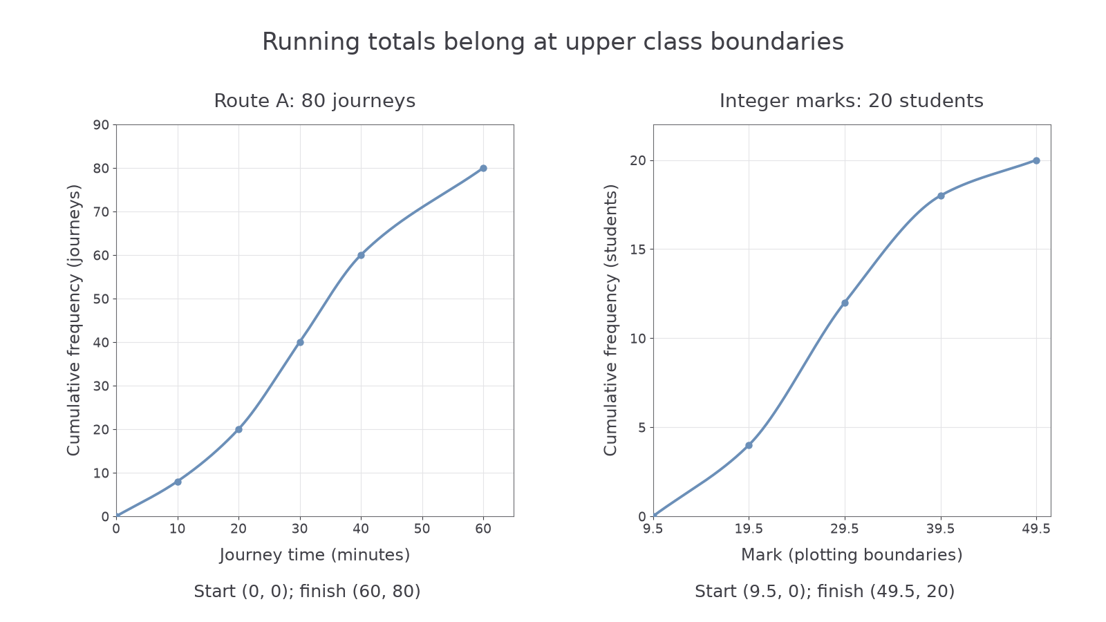
The totals are $8$, $8+12=20$, then $40,60,80$. Begin at $(0,0)$; plot $(10,8),(20,20),(30,40),(40,60),(60,80)$. Draw a non-decreasing curve through the points, as in the left construction diagram.

Answer. The cumulative table is shown above; the graph finishes at $(60,80)$.

Check. Consecutive total differences recover $8,12,20,20,20$. Their sum is eighty, matching the graph's final height. Plotting $(25,40)$ instead of $(30,40)$ would wrongly use a class midpoint.

Worked example 2: grouped integer marks

Question. Integer marks are grouped as ten–nineteen, twenty–twenty-nine, thirty–thirty-nine and forty–forty-nine, with frequencies $4,8,6,2$. Give cumulative graph coordinates using continuous plotting boundaries.

Plan. Use halfway boundaries that separate adjacent integer groups, then accumulate the frequencies.

The upper boundaries are $19.5,29.5,39.5,49.5$, with first lower boundary $9.5$. The totals are $4,12,18,20$.

Answer. Start at $(9.5,0)$, then plot $(19.5,4),(29.5,12),(39.5,18),(49.5,20)$, and join with a non-decreasing curve.

Check. The increment from twelve to eighteen is six, recovering the third class. Halfway boundaries keep the adjacent integer groups separate; they do not claim that a student actually scored a fractional mark.

Watch out

A cumulative graph can stay level if a class is empty, but it cannot decrease. Check its final height against the sum of the class frequencies.

Quartiles from a grouped cumulative curve

For total frequency $N$, estimate the lower quartile $Q_1$, median and upper quartile $Q_3$ at cumulative heights $N/4$, $N/2$ and $3N/4$. These divide the modelled distribution into quarters. The interquartile range, $IQR=Q_3-Q_1$, measures the spread of the middle half of the data in the original measurement units.

Worked example 3: quartiles at plotted boundaries

Question. Estimate Route A's quartiles, median and IQR from its cumulative curve.

Plan. Use the total eighty to find the three vertical reading levels.

Reading across and down gives $Q_1=20$ minutes, median $30$ minutes and $Q_3=40$ minutes. Thus $IQR=40-20=20$ minutes.

Answer. Lower quartile about twenty minutes, median thirty minutes, upper quartile forty minutes; IQR twenty minutes.

Check. The original running totals at times twenty, thirty and forty are exactly twenty, forty and sixty, so the readings agree with the table. The quartile times are ordered around the median, and the IQR has units of minutes rather than people.

Worked example 4: specified straight-line interpolation

Question. Sixty clinic waits have class boundaries $0,10,20,30,40$ minutes and class frequencies $6,18,24,12$. Using straight-line interpolation between cumulative points, estimate all three quartiles and the IQR.

Plan. Form cumulative totals $0,6,24,48,60$. Find heights fifteen, thirty and forty-five, then locate each proportionally within its class.

For $Q_1$, height fifteen is nine above six, out of the next class's eighteen:

For the median and upper quartile, start at twenty minutes, where the cumulative total is twenty-four:

Answer. $Q_1\approx15$, median $\approx22.5$, $Q_3\approx28.75$ minutes; $IQR\approx28.75-15=13.75$ minutes.

Check. At fifteen minutes the model has accumulated $6+9=15$. At $22.5$, one quarter of the twenty-four-observation class adds six, giving thirty. At $28.75$, seven eighths of that class adds twenty-one, giving forty-five. These recover the required cumulative levels independently.