FA13, HA14 - Graphs in real situations | Eduqas GCSE Mathematics

A horizontal travel graph can represent a long stop, while a steep graph can represent fast movement. FA13 and HA14 connect graphs, including reciprocal and non-standard models, to quantities such as distance, time and speed. Read approximate solutions with units and use the supplied constant-acceleration formulae where their conditions apply.

Distance-time graphs

If a travel graph becomes horizontal, has the traveller slowed down or stopped? Check the vertical quantity: if distance stays unchanged while time passes, the traveller is stationary.

On a straight segment of a distance-time graph, speed is the magnitude of the distance change divided by the time change. A steeper segment means a greater speed when comparing on the same axes and scales. A straight sloping segment represents constant speed; a horizontal segment represents a stop.

Distance labels matter

A graph of total distance travelled never falls. A graph of distance from a starting point can fall when the traveller returns towards the start. On a straight route, a falling segment's negative gradient shows the return direction; its speed is the positive magnitude of that gradient.

Read elapsed time by subtraction. For example, between 10:40 and 11:10 there are 30 minutes, not 70 minutes. Match the time unit to the speed unit before dividing.

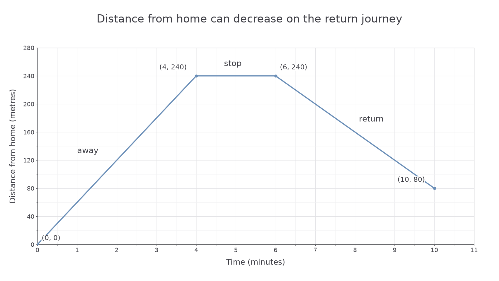
[DIAGRAM: asset_name: A journey away and partly back; asset_slug: distance-time-journey; caption: A rising segment, a stop and a return segment have different meanings.; description: A scaled graph of distance from home in metres against time in minutes joins (0,0), (4,240), (6,240) and (10,80), with all four points labelled.]

Worked example 1: travelling and stopping

Question. A walker is $240\,\mathrm m$ from home after four minutes, remains there until minute six, then walks back along the same straight route. Find the outward speed and the length of the stop.

Plan. Use the rising segment's distance change and the horizontal segment's duration.

\begin{aligned} \text{outward speed}&=\frac{240-0}{4-0}=60\,\mathrm{m/min}\\ \text{stop duration}&=6-4=2\text{ minutes} \end{aligned}

Answer. $60\,\mathrm{m/min}$ ; a two-minute stop.

Check. Four minutes at $60\,\mathrm{m/min}$ covers $240\,\mathrm m$ . During the stop the height stays $240\,\mathrm m$ , rather than falling to zero.

Now interpret the falling segment and distinguish distance travelled from final distance from home.

Worked example 2: a return journey

Question. In the same journey, the walker is $80\,\mathrm m$ from home at minute ten. Find the return speed and average speed over the whole ten minutes, including the stop.

Plan. Use the fall in distance for the return segment, then add actual distances for the whole journey.

\begin{aligned} \text{return speed}&=\frac{240-80}{10-6}=40\,\mathrm{m/min}\\ \text{total distance}&=240+(240-80)=400\,\mathrm m\\ \text{average speed}&=\frac{400}{10}=40\,\mathrm{m/min} \end{aligned}

Answer. Return speed $40\,\mathrm{m/min}$ ; whole-journey average $40\,\mathrm{m/min}$ .

Check. The graph's return gradient is $-40\,\mathrm{m/min}$ , showing decreasing distance from home. Speed is positive. Dividing the final height $80$ by ten would ignore the outward and return distances.

Speed belongs to a time interval, not just one plotted height.

Watch out

A point at height $240\,\mathrm m$ does not mean speed $240\,\mathrm{m/min}$ . Height gives distance; the change in height divided by elapsed time gives speed on a straight segment.

Read a fresh return segment from complete data.

Other real graphs

Some real relationships are curved because equal input changes do not produce equal output changes. Start with the quantities, units and allowed inputs, then calculate a table from the model.

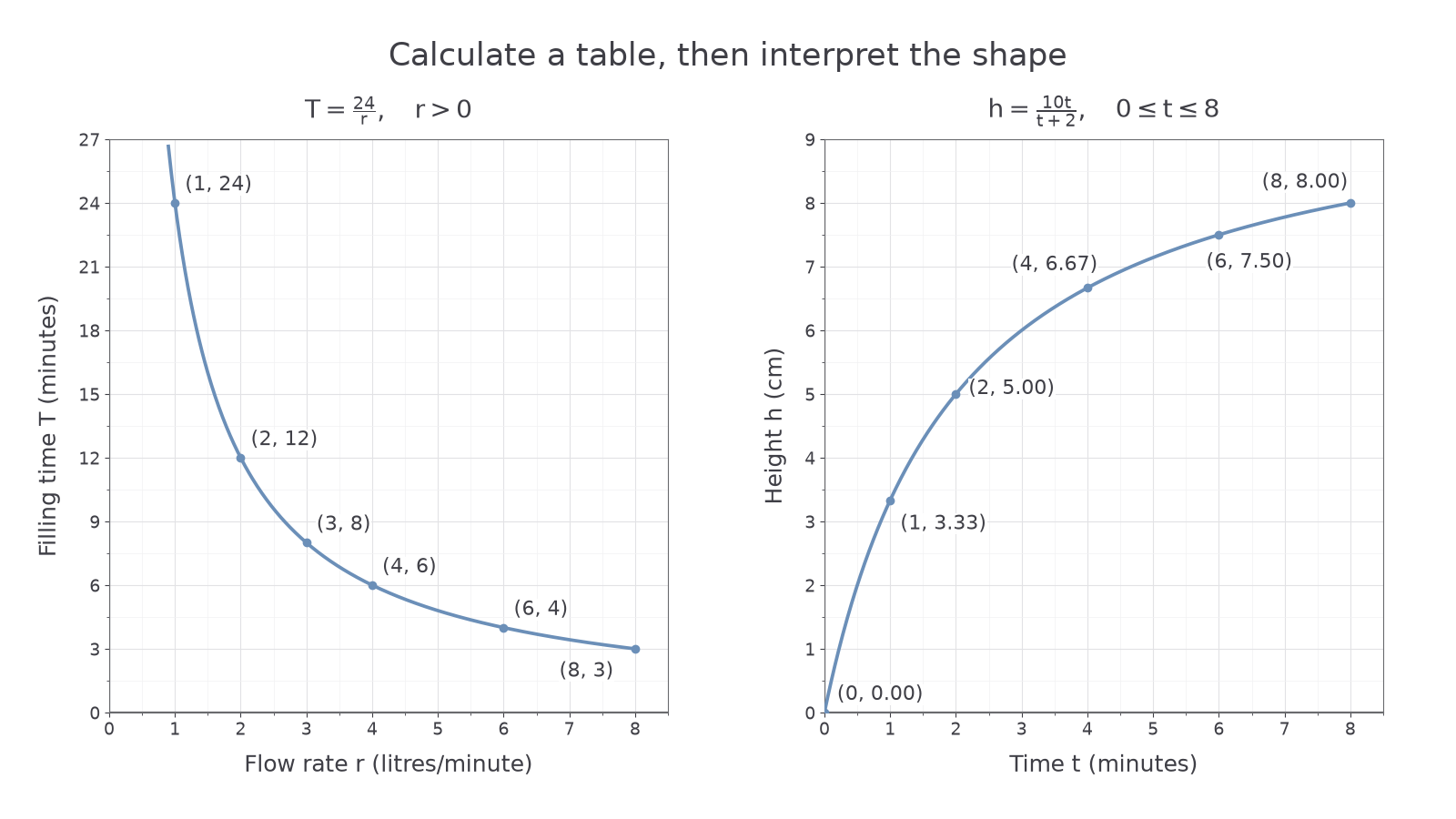
For a fixed $24\,\mathrm L$ volume, a flow rate $r\,\mathrm{L/min}$ gives filling time $T=24/r$ minutes. The reciprocal shape expresses a practical trade-off: double the rate and the filling time halves. Rates must be positive, so only the positive branch describes this situation.

[DIAGRAM: asset_name: Reciprocal and non-standard real models; asset_slug: real-model-curves; caption: A positive reciprocal model falls, while a different supplied model can rise and flatten.; description: Left scaled grid plots filling time T equals 24 divided by flow rate r for positive r up to 8 litres per minute. Right scaled grid plots h equals 10t divided by t plus 2 for times from 0 to 8 minutes, with table points labelled and height in centimetres.]
A positive reciprocal model falls, while a different supplied model can rise and flatten.

Worked example 3: plotting a reciprocal model

Question. Plot the filling-time model $T=24/r$ for rates from $1$ to $8\,\mathrm{L/min}$ . Find the time at $r=3$ and $r=6$ .

Plan. Divide the fixed volume by each rate and plot the pairs with rate horizontally.

$r$ , $\mathrm{L/min}$	$1$	$2$	$3$	$4$	$6$	$8$
$T$ , minutes	$24$	$12$	$8$	$6$	$4$	$3$

Answer. A smooth decreasing curve; eight minutes at $3\,\mathrm{L/min}$ , four minutes at $6\,\mathrm{L/min}$ .

Check. $3(8)=24$ and $6(4)=24$ litres. A negative rate and time would not describe this filling process, despite belonging to the unrestricted algebraic reciprocal graph.

The next rule is supplied explicitly. You can plot an unfamiliar formula without first memorising its shape.

Worked example 4: a non-standard model

Question. A liquid-height model is $h=\frac{10t}{t+2}$ , with $h$ in centimetres and $0\le t\le8$ minutes. Calculate a table and describe the graph's change.

Plan. Substitute the times into both numerator and denominator, then draw a smooth curve.

At $t=4$ , $h=40/(4+2)=40/6\approx6.67\,\mathrm{cm}$ .

$t$ , minutes	$0$	$1$	$2$	$4$	$6$	$8$
$h$ , cm	$0$	$3.33$	$5$	$6.67$	$7.5$	$8$

Answer. The height rises quickly at first, then rises more slowly; the curve flattens over the stated interval.

Check. Over equal two-minute intervals, the rises from minute two onwards are about $1.67$ , $0.83$ and $0.50\,\mathrm{cm}$ . These decreasing rises agree with the flattening curve. The model is only asserted from zero to eight minutes.

The allowed inputs form the model's domain. Zero flow is excluded in the filling model because it gives no finite filling time. Zero time is allowed in the height model and gives the initial height zero. Always examine the actual denominator and context rather than exclude zero from every curved graph.

Watch out

Doubling flow does not double filling time. For a fixed volume, $T=V/r$ , so doubling the denominator halves the time. The falling reciprocal curve reflects this.

Use the reciprocal model with new values.

Continue this lesson.

You’re previewing NovaLearn without an account. Create a free account to read the rest.

Create free account

Last Accessed

Number

Algebra

Ratio and proportion

Geometry and measures

Higher graphs

Probability

Statistics

FA13, HA14 - Graphs in real situations

Distance-time graphs

Other real graphs

Continue this lesson.

Learn faster with Nova