FS6, HS7 - Scatter graphs and prediction
A line of best fit predicts a typical outcome. Does its prediction apply exactly to every individual? FS6 and HS7 use paired observations to describe relationships, estimate within a trend, and judge when a prediction goes beyond the evidence.
Bivariate data
Each plotted point must keep two measurements from the same person or item together. Swapping which measurements belong together changes the relationship.
Bivariate data and correlation
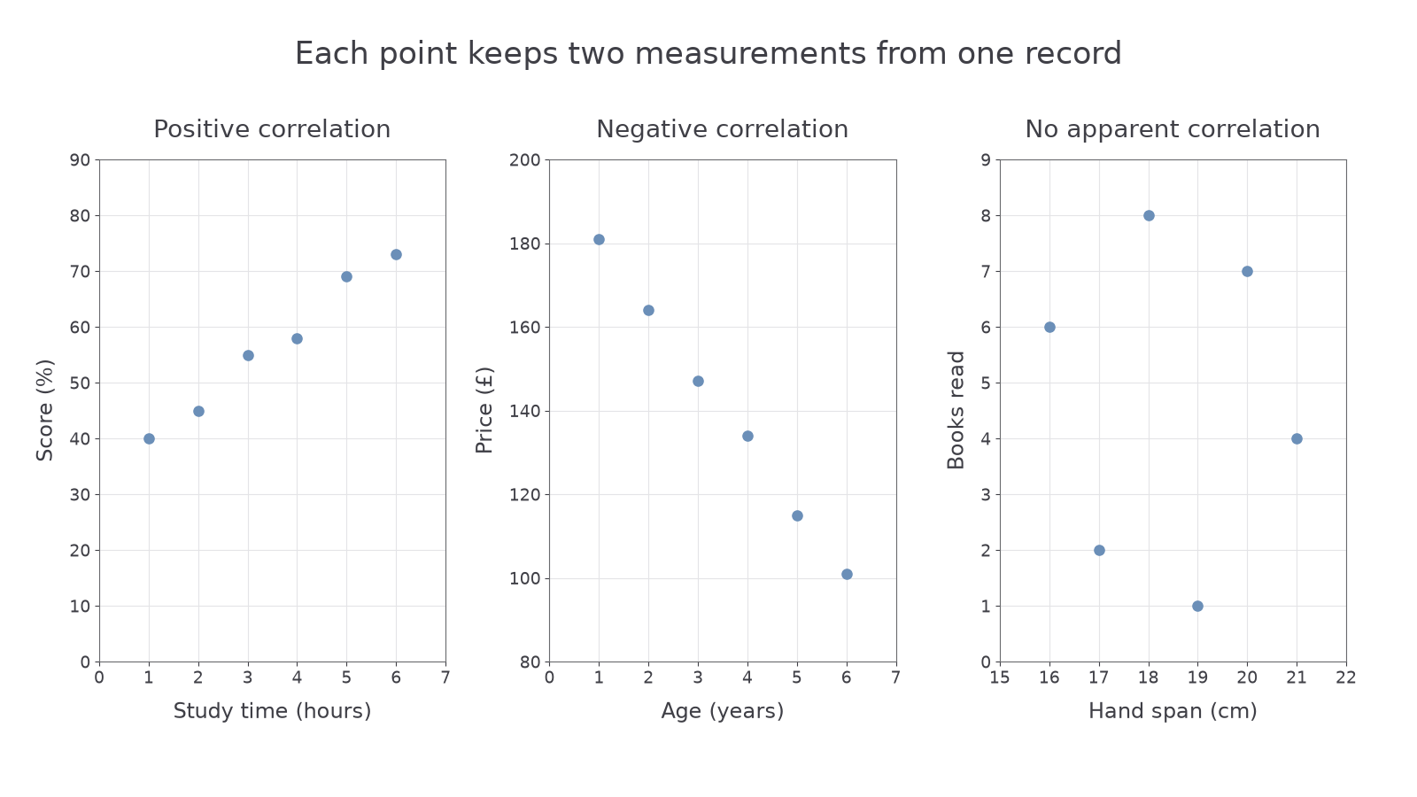
Bivariate data records two variables for each individual or item. A scatter graph plots each pair as one point. Positive correlation means larger values of one variable tend to accompany larger values of the other; negative correlation means they tend to accompany smaller values. No apparent correlation means there is no clear increasing or decreasing trend. The closer the points lie to a clear trend, the stronger that correlation.
Choose labelled numerical axes with units and uniform scales. Put each pair in the correct horizontal and vertical position. Do not join consecutive points: their row order is not a time-series path. Keep the paired rows intact; sorting each column separately would invent new pairs.
Worked example 1: plotting a positive relationship
Question. Plot these six learners' study times and test scores, and describe the association.
| Study time (hours) | ||||||
|---|---|---|---|---|---|---|
| Score (%) |
Plan. Use study time on the horizontal axis and score on the vertical axis; plot one point per learner.
For the fourth learner, move across to four hours and up to , marking . Plot the remaining pairs in the same way. In the left panel below, the cloud rises from left to right, with some scatter rather than a perfect line.
Answer. There is a clear positive correlation: learners with longer study times tend to have higher scores in these data.
Check. There are six plotted points for six paired records. The points and match the first and last rows, and the fourth point has not been reversed to .
A downward trend has the opposite direction; scattered points without either trend need a different description.
Worked example 2: plotting a negative relationship
Question. Plot these used phones' ages and selling prices, then describe the correlation.
| Age (years) | ||||||
|---|---|---|---|---|---|---|
| Price (£) |
Plan. Put age on the horizontal axis and price on the vertical axis, keeping every age with its own price.
For example, the four-year-old phone gives point . The points move generally downwards as age increases, as in the centre panel.
Answer. Negative correlation: older phones tend to sell for less in this sample.
Check. The youngest and oldest records plot at , ; the intermediate points also follow the downward pattern. A negative correlation describes the direction of association, not a negative selling price.
The right panel uses hand spans cm paired with books read in a month. Neither larger nor smaller book counts consistently accompany larger spans, so there is no apparent correlation. This does not prove that every possible kind of relationship is absent; it describes the lack of a clear trend in these observations.
[DIAGRAM: asset_name: Three scatter patterns; asset_slug: scatter-correlation-patterns; caption: Paired points can show positive, negative or no apparent correlation.; description: Three labelled scaled scatter plots use exactly the study-time/score pairs, phone-age/price pairs and hand-span/books pairs in the teaching. The first rises, the second falls and the third has no clear trend. Points are not joined.]
Watch out
Use the variables in your description: “price tends to decrease as age increases” communicates more than the word “negative” alone. A trend does not require every successive pair to move in exactly the same direction.
Read a pair and describe a fresh trend.
Lines of best fit
A representative line summarises a roughly straight trend. It should run through the middle of the cloud, with points reasonably balanced above and below across the observed range.
Best fit and interpolation
An estimated line of best fit represents the overall linear trend; it need not pass through actual data points or the origin. Interpolation predicts within the range supported by the observed data. Read from an input to the line, then across to the other axis. A prediction estimates an outcome, rather than reproducing every observation.
Do not join the first and last plotted points automatically. Use all the points to judge the line, allowing for the scatter. Different reasonable lines drawn by eye can give slightly different estimates; report suitable precision. If there is no useful trend, a straight line provides little basis for prediction.
Worked example 3: a forward prediction
Question. For the study data, a representative line is , where is study time in hours and is predicted score in percent. Estimate a score for hours, to the nearest whole percent.
Plan. Move vertically from to the chosen line and horizontally to the score axis; use its equation to check the reading.
The left fit diagram gives a height of about . From the rule,
The time lies inside the observed one-to-six-hour range, so this is interpolation.
Answer. A predicted score of about .
Check. The chosen line has heights at three hours and at four. Halfway between those heights is , matching the calculation. These are line heights; the actual observations need not equal them.
You can also read from a known vertical-axis value towards the horizontal axis.
Worked example 4: a reverse prediction
Question. A representative line for the phone data is , with age in years and predicted price in pounds. Estimate the age corresponding to .
Plan. Move horizontally from to the line, then vertically down to age, or rearrange the line equation.
This age is within the observed one-to-six-year range.
Answer. About years, an interpolated estimate.
Check. The line predicts at two years and at three; is halfway between them, so the age estimate is halfway as well. The data do not guarantee that every phone selling for this price has that age.
Continue this lesson.
You’re previewing NovaLearn without an account. Create a free account to read the rest.
Create free account