FS3–FS4, HS3, HS5 - Discrete and time-series graphs

Discrete numerical data

Discrete numerical data take separate allowed values, such as the number of pets in a household: $0,1,2,\ldots$. A count cannot be $1.7$ pets. Discrete values need not always be whole numbers: shoe sizes can occur in fixed half-size steps.

Worked example 1: constructing vertical lines

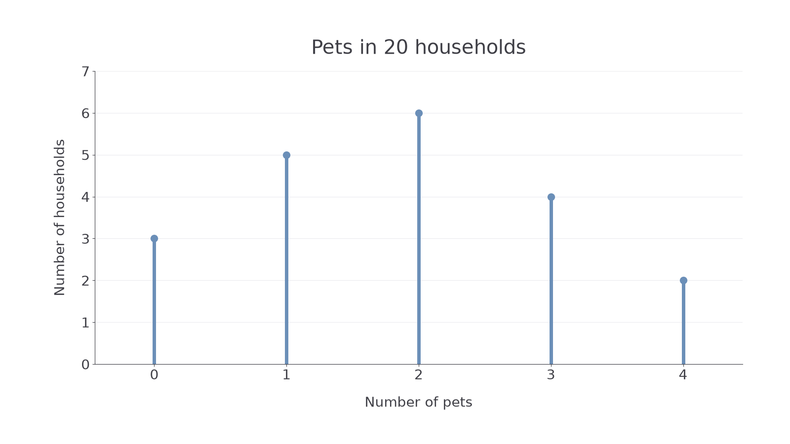
Question. Twenty households report their number of pets as follows. Describe a suitable vertical-line chart and find the number with at least $3$ pets.

Plan. Put the pet counts on the horizontal numerical axis; use household frequencies for line heights.

Draw lines at $0,1,2,3,4$ reaching heights $3,5,6,4,2$. Label the axes “Number of pets” and “Number of households”.

Answer. The chart below displays the table. At least $3$ pets means $3$ or $4$, so $4+2=6$ households.

Check. All frequencies total $3+5+6+4+2=20$. The other $14$ households have fewer than $3$ pets.

Worked example 2: preserving numerical gaps

Question. Nine pupils borrow $0$, $2$ or $5$ books, with respective frequencies $4,3,2$. How should these be placed on a vertical-line chart?

Plan. Use a genuine number scale, keeping every unit interval the same width.

Mark $0,1,2,3,4,5$ at equal intervals. Draw a line of height $4$ at $0$, height $3$ at $2$ and height $2$ at $5$. Values $1,3,4$ have zero frequency, so no raised line is needed there.

Answer. The gap from $2$ to $5$ is three times the gap from $0$ to $1$, and the lines are not equally spaced as three category labels.

Check. Frequencies $4+3+2=9$ account for every pupil. Equal spacing of just the three observed labels would falsely suggest equal numerical gaps.

Which axis is which?

The value $2$ pets is a possible observation. The frequency $6$ says how many households have that value. Interchanging them changes the meaning of the chart.

Time-series line graph

Plot each observation at its time and join successive observations with straight segments to show how the recorded quantity changes over time. Equal time intervals must occupy equal horizontal distances.

Worked example 3: plotting from a table

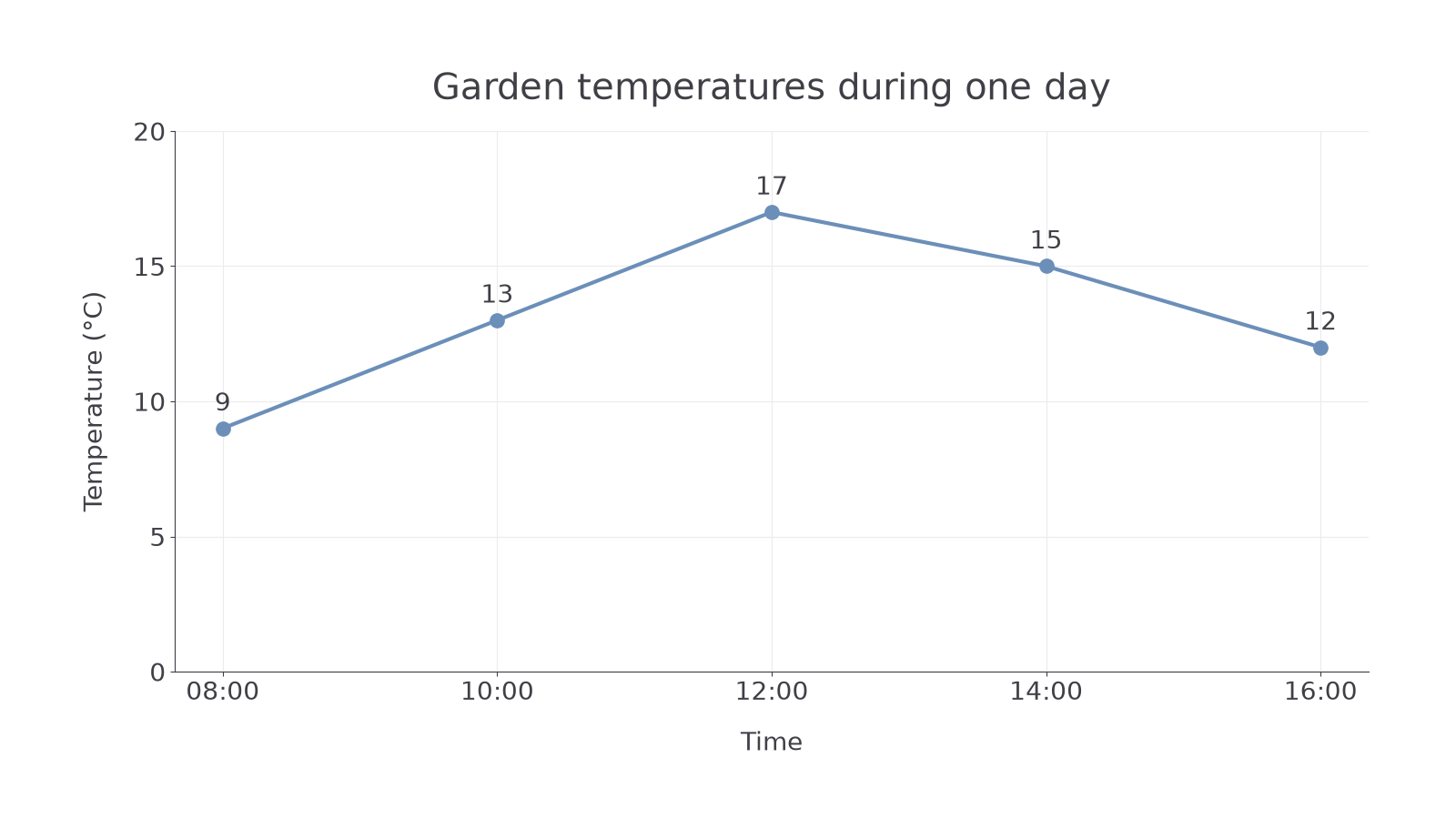
Question. A gardener records these temperatures. Construct a time-series graph and describe the changes.

Plan. Use equally spaced two-hour positions, plot the temperature at each time and join consecutive points.

Choose a vertical scale $0$ to $20\,^\circ\mathrm C$ in steps of $5\,^\circ\mathrm C$. Plot the five points shown below.

Answer. The recorded temperature rises from $9\,^\circ\mathrm C$ to $17\,^\circ\mathrm C$, then falls to $12\,^\circ\mathrm C$. The highest recorded value is at $12{:}00$.

Check. Reading the plotted points back in time order reproduces $9,13,17,15,12$. The overall recorded change is $12-9=3\,^\circ\mathrm C$, although the temperature did not rise throughout.

Worked example 4: unequal time intervals

Question. A room has temperatures $8\,^\circ\mathrm C$ at $09{:}00$, $10\,^\circ\mathrm C$ at $10{:}00$ and $9\,^\circ\mathrm C$ at $12{:}00$. Explain how to space the times and estimate the temperature at $11{:}00$ using straight segments.

Plan. Space points by elapsed time, then use the position halfway through the two-hour final interval.

The $10{:}00$ to $12{:}00$ gap is twice the $09{:}00$ to $10{:}00$ gap. $11{:}00$ is halfway from $10{:}00$ to $12{:}00$, so its straight-line estimate is

Answer. Use horizontal gaps in the ratio $1:2$; the estimate is $9.5\,^\circ\mathrm C$.

Check. $9.5$ is halfway between $9$ and $10$. The actual temperature could have fluctuated between readings, so this value is not an observed fact.