HA14–HA15, HR16 - Rates and areas under graphs

Tangents and chords

A curved distance-time graph gets steeper as time passes. Does one average speed describe how fast the object is moving at every instant? An interval's average and a single instant's rate answer different questions.

A chord joins two selected points of a curve. Its gradient gives the average rate over their input interval:

A tangent follows a smooth curve's local direction at a chosen point. Its gradient gives the instantaneous rate there. For a general curve, a tangent may cross the curve or meet it again elsewhere; the local direction is what matters.

A long gradient triangle reduces the effect of small reading errors. A line from the origin to the selected curve point is usually a chord, not its tangent. For a distance in metres and time in seconds, both average speed and instantaneous speed have units $\text{m/s}$.

Keep the curve and interval average, but move the chosen instant later, to a steeper point.

The diagrams distinguish the curve, its interval chord and the tangents at the two instants.

[DIAGRAM: asset_name: Chord and tangent rates; asset_slug: chord-tangent-rates; caption: An interval chord gives an average; a tangent gives the rate at its contact time.; description: Exact distance curve d=t squared over0to6 seconds is shown with the chord from(1,1) to(4,16) and tangent at3 through(2,3),(4,15). Second panel shows tangent at4 through(2,0),(6,32). Axes show metres and seconds; read-off points on tangents are distinct from the contact points.]

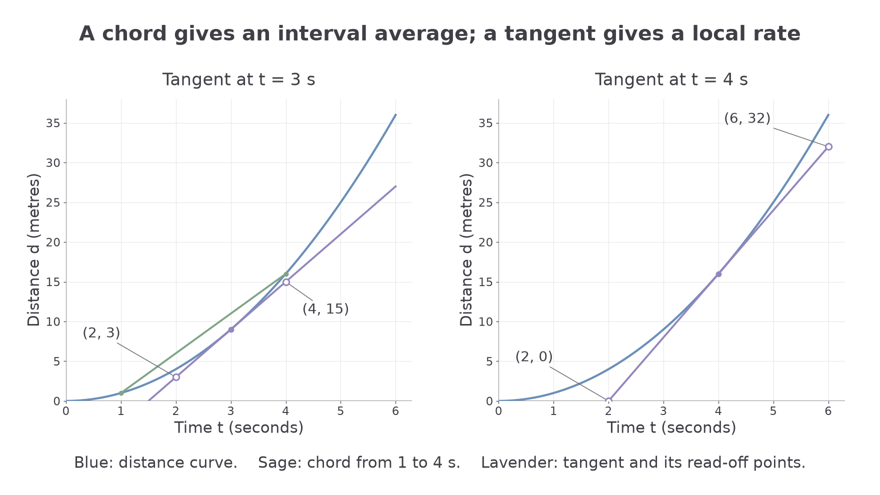
The drawn-tangent method estimates the rate: its accuracy depends on the curve, line placement and coordinate readings. A negative gradient means the output is decreasing, not that its value is necessarily negative. Keep the sign of a rate of change; a falling water level, for example, has a negative depth-time gradient.

The supplied constant-acceleration equations can also model motion when acceleration is constant; establish that condition before using them. A curved distance-time graph alone does not establish constant acceleration.

Distinguish a fresh interval average from a tangent estimate.

Areas under graphs

For constant speed, distance equals speed multiplied by time: the area of a rectangle under a speed-time graph. If speed varies, divide the interval into strips and add the approximate distances. This explains why an area can represent an accumulated quantity.

A straight line between two readings creates a trapezium. For width $h$ and endpoint heights $u,v$, its area is

Add the separate trapezium areas. With unequal input intervals, use each strip's own width. For a curved graph these straight-edged strips generally give an estimate, even when the reading arithmetic is exact.

Here a speed curve $v=t^2+2$, with seconds and metres per second, is estimated over $0\le t\le4$.

Keep the curve and time interval, but use more readings and narrower strips.

On this upward-bending curve, the joining chords lie above the curve, so both trapezium sums overestimate the actual area. The narrower strips follow the curve more closely. On a downward-bending section the chord strips lie below, giving an underestimate instead; a curve with changing curvature requires separate consideration.

[DIAGRAM: asset_name: Coarse and fine area estimates; asset_slug: trapezium-refinement; caption: Narrower strips track the same curve more closely; both sums remain estimates.; description: Exact speed curve v=t squared+2 from0to4 is compared with two width2 trapezia and four width1 trapezia. Pale fills show chord-edged areas above the upward-bending curve; totals32m and30m and the true curve are clearly distinguished.]

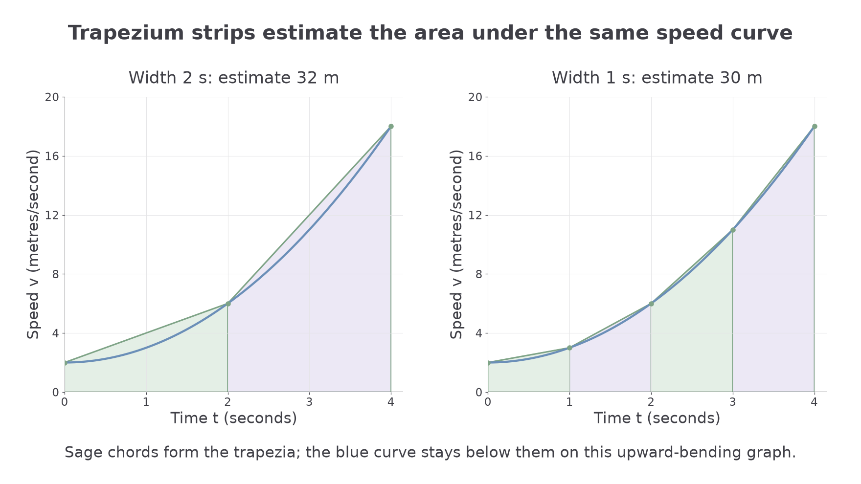
More, narrower strips usually improve an estimate for a smooth curve, but precision is still limited by the graph and readings. Use sensible reported accuracy. A finite decimal produced by the strip arithmetic does not make the curved area exact. If the graph is genuinely made of straight segments, suitable triangles, rectangles and trapezia can give its area exactly.

For a region between two graphs, use their vertical separation as the strip height. Subtract the lower ordinate from the upper at each input, then form trapezia. Equivalently, estimate both areas from the same baseline and subtract, using the same interval and subdivisions.