6.1, 6.2 - Cumulative frequency and estimated quartiles

Build a cumulative-frequency diagram from grouped data, then use it to estimate a median, quartiles and counts above or between limits. You will distinguish recorded class totals from estimates inside classes.

Cumulative totals and boundaries (Higher)

A teacher knows only grouped completion times for $60$ pupils. Can we still estimate the time by which half finished, and how many took longer than $35$ minutes?

You already know

A median divides ordered data into halves. Lower and upper quartiles locate its quarter and three-quarter points; their difference is the interquartile range, or IQR.

A running count keeps everyone already counted when a new class is added. It cannot decrease as the time limit increases.

Cumulative frequency

The number of observations up to a specified boundary. It adds the current class frequency to all preceding frequencies.

Use the table's endpoint convention. With $0<t\leq10$ , $10<t\leq20$ , the total at $20$ counts $t\leq20$ . For classes $0\leq t<10$ , $10\leq t<20$ , it instead counts $t<20$ . Do not count a shared boundary twice.

Worked example 1: build the running totals

Question. Complete the cumulative frequencies for these task times.

Time $t$ in minutes	Frequency	Cumulative frequency
$0<t\leq10$	$8$	?
$10<t\leq20$	$12$	?
$20<t\leq30$	$20$	?
$30<t\leq40$	$8$	?
$40<t\leq60$	$12$	?

Plan. Add each frequency to the total so far.

\begin{aligned} C(10)&=8 &&\text{first class}\\ C(20)&=8+12=20 &&\text{first two classes}\\ C(30)&=20+20=40 &&\text{include the third}\\ C(40)&=40+8=48 &&\text{include the fourth}\\ C(60)&=48+12=60 &&\text{all pupils} \end{aligned}

Why is $C(30)=40$ , not $20$ ? It includes everyone taking at most $30$ minutes, rather than just the last class.

Answer. The running totals are $8,20,40,48,60$ .

Check. Consecutive differences recover $8,12,20,8,12$ .

Change only the last class frequency from $12$ to $24$ . The earlier totals must stay fixed.

Worked example 2: change the final class

Question. Find the revised cumulative frequencies and total number of pupils.

Plan. Keep totals up to $40$ minutes and add the revised final frequency.

\begin{aligned} C(10),C(20),C(30),C(40)&=8,20,40,48 &&\text{earlier classes unchanged}\\ C(60)&=48+24=72 &&\text{new final class} \end{aligned}

Why do earlier totals not change? The extra pupils all took more than $40$ minutes.

Answer. $8,20,40,48,72$ ; there are $72$ pupils.

Check. $72-48=24$ , the revised final frequency.

A surprising consequence follows: adding only slow finishers can move the median, even though every faster pupil's time stays the same. The median's target position depends on the whole group size.

Watch out

The line $C(20)=12$ gives one class frequency. The correct running total is $8+12=20$ .

For the check, start the running total afresh rather than carrying over a number from the examples.

Constructing cumulative-frequency diagrams (Higher)

Plot the measured variable horizontally and cumulative frequency vertically, using upper boundaries rather than midpoints.

At an upper boundary, the full class has been counted. At its midpoint, only part of the class has been reached, and its exact count is unknown. Include a zero-frequency starting point at the first lower boundary when no observations lie below it. Choose uniform scales covering the full interval and total.

Worked example 3: plot the original table

Question. Construct the diagram for the original $60$ -pupil table, using straight joins.

Plan. Pair each upper boundary with its running total and add the lower-boundary zero point.

\begin{aligned} \text{start}&:(0,0) &&\text{no positive time below zero}\\ \text{first points}&:(10,8),(20,20),(30,40) &&\text{upper boundaries and totals}\\ \text{last points}&:(40,48),(60,60) &&\text{complete the table} \end{aligned}

Why use $(20,20)$ , not $(15,20)$ ? The running total $20$ applies at the class endpoint $20$ minutes.

Answer. Plot these points and join consecutive points with straight segments.

[DIAGRAM: asset_slug: m088_cumulative; caption: Completion-time cumulative-frequency diagram for sixty pupils using upper boundaries and straight joins; description: Points zero zero, ten eight, twenty twenty, thirty forty, forty forty-eight and sixty sixty with time in minutes horizontally; file: m088_cumulative.png; recommended_method: matplotlib]
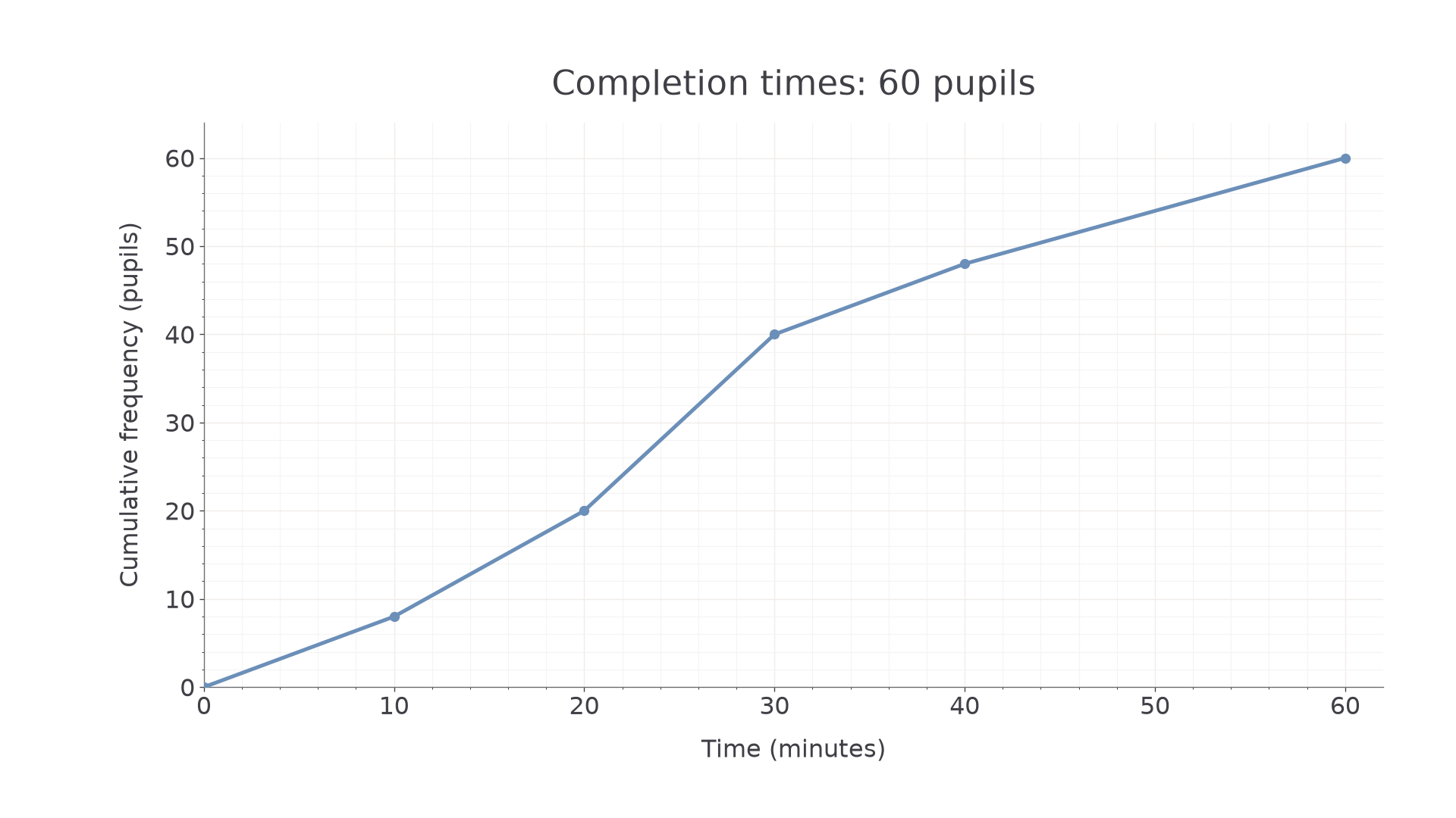
Completion-time cumulative-frequency diagram for sixty pupils using upper boundaries and straight joins

Check. The graph never falls and ends at $(60,60)$ , representing every pupil.

Change only the final frequency to $24$ , as in Worked example $2$ . The graph changes only after $40$ minutes.

Worked example 4: plot the revised final total

Question. Construct the diagram for the revised $72$ -pupil table.

Plan. Retain the points through $(40,48)$ , then use the new final total.

\begin{aligned} \text{unchanged points}&:(0,0),(10,8),(20,20),(30,40),(40,48) &&\text{same earlier totals}\\ \text{new endpoint}&:(60,72) &&\text{all revised observations} \end{aligned}

Why does the last segment rise more steeply? It now adds $24$ , rather than $12$ , pupils over the same time width.

Answer. The revised diagram is below.

[DIAGRAM: asset_slug: m088_more_pupils; caption: Revised cumulative-frequency diagram after changing only the last class frequency; description: Earlier points unchanged through forty minutes and cumulative forty-eight, then the final point is sixty minutes and seventy-two pupils; file: m088_more_pupils.png; recommended_method: matplotlib]

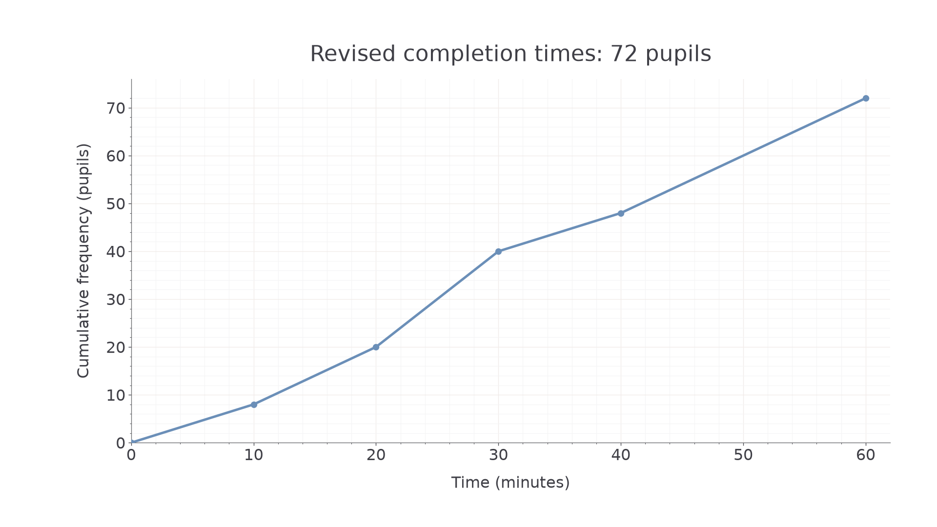
Check. The last rise is $72-48=24$ , matching the changed class.

Pearson diagrams may be joined by a smooth nondecreasing curve or suitable straight segments. Follow any stated instruction; do not draw a line of best fit. Here all joins are straight. This fixes a linear interpolation model: within a class, equal time widths contain equal estimated shares of the frequency. A zero-frequency class would give a horizontal segment.

Watch out

Plotting $(15,20)$ puts the second running total at a midpoint. Correct it to $(20,20)$ , the upper boundary. Separate bars or a staircase do not provide the intended interpolation diagram.

The next table has a wider last interval. Its horizontal distance must be drawn to scale.

Estimating the median and quartiles (Higher)

Locate a fraction of the total on the cumulative-frequency axis, move across to the graph, then down to read a time.

For total $N$ , the lower quartile uses $N/4$ , the median uses $N/2$ , and the upper quartile uses $3N/4$ . These are cumulative counts, not times. The IQR is the difference between the upper and lower quartile time readings.

Cumulative quartile levels

Q_1:\frac N4\qquad \text{median}:\frac N2\qquad Q_3:\frac{3N}{4}

\mathrm{IQR}=Q_3-Q_1

Not in the Higher formulae sheet: learn these relationships.

Last Accessed

Number

Algebra

Shape, space and measure

Handling data

6.1, 6.2 - Cumulative frequency and estimated quartiles

Cumulative totals and boundaries (Higher)

Constructing cumulative-frequency diagrams (Higher)

Estimating the median and quartiles (Higher)

Continue this lesson.

Learn faster with Nova