3.3 - Cubic and reciprocal graphs

Cubic and reciprocal graphs can bend, turn or split into separate branches. You will use tables, signs and excluded inputs to recognise and draw their actual shapes, including equations with different variable letters. Checking the equation first prevents a familiar-looking curve from leading you astray.

Plotting cubic graphs (Higher)

At $x=2$ , both $y=2/x$ and $y=4/x^2$ give $y=1$ . Will they still agree at $x=-2$ ? By the end, the signs and shapes of the graphs will make the answer clear. First, consider curves with no division at all.

You already know

Substitute an input into every term, putting negative values in brackets. Curved graphs need smooth curves through their plotted points, not ruler segments.

A cubic polynomial has highest power $3$ , with a nonzero coefficient of the cubed term. The simplest graph, $y=x^3$ , passes through the origin in an increasing S shape. Other terms can create two changes of direction and three x-axis crossings, so not every cubic has the same simple shape.

Polynomial graph family

y=Ax^3+Bx^2+Cx+D

Here the constants are integers and some may be zero. The variables may use other letters. If $A=0$ , the degree reduces; the expression is no longer cubic. Not in the Higher formulae sheet: learn to recognise the form.

There is no denominator, so every real input is allowed algebraically. A question may still restrict the interval to be drawn. That drawing interval is different from an input excluded because an expression is undefined. For a cubic, a positive leading coefficient makes the far-left end low and far-right end high; a negative one reverses those end directions.

Worked example 1: a cubic with three crossings

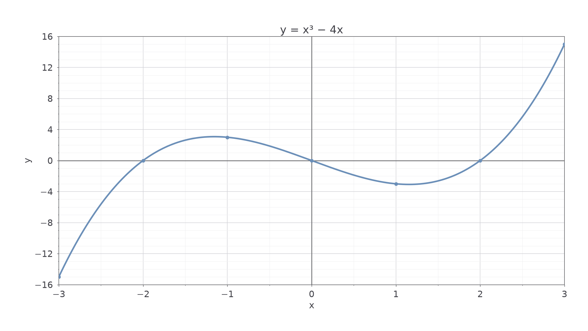
Question. Draw $y=x^3-4x$ for $-3\leq x\leq3$ , showing its x-axis crossings.

Plan. Calculate a table, check the zeros by factorising, then draw a smooth curve through the points.

\begin{aligned} x=-1&:\quad y=(-1)^3-4(-1)=3 &&\text{substitute with brackets}\\ y&=x(x^2-4)=x(x-2)(x+2) &&\text{factorise to check the zeros} \end{aligned}

$x$	$-3$	$-2$	$-1$	$0$	$1$	$2$	$3$
$y$	$-15$	$0$	$3$	$0$	$-3$	$0$	$15$

Use regular scales reaching all the listed outputs. Plot the points, then join smoothly, keeping the two changes of direction visible.

Why? The positive output between $-2$ and $0$ , then the negative output between $0$ and $2$ , prevents us drawing one continuously rising S.

Answer. The graph below crosses at $(-2,0)$ , $(0,0)$ and $(2,0)$ .

Check. Each crossing makes a factor zero. Opposite inputs in the table give opposite outputs.

That last check reveals a striking symmetry: a half-turn about the origin takes this graph onto itself. Substituting $-x$ into $x^3-4x$ gives the negative of the original output. This is not symmetry about the vertical axis.

[DIAGRAM: asset_slug: m051_cubic; caption: A cubic with three x-intercepts and two changes of direction; description: Exact graph y equals x cubed minus 4x over negative 3 to 3, crossing the horizontal axis at negative 2, 0 and 2; file: m051_cubic.png; recommended_method: matplotlib]

Change only the coefficient of $x$ , from $-4$ to $-1$ . The turns become smaller, so half-integer inputs help reveal them.

Worked example 2: do not miss small turns

Question. Draw $y=x^3-x$ for $-2\leq x\leq2$ , showing its x-axis crossings.

Plan. Include inputs between the integer zeros, then draw a smooth curve through all the points.

\begin{aligned} x=-0.5&:\quad y=(-0.5)^3-(-0.5)=0.375 &&\text{look between zeros}\\ x=0.5&:\quad y=0.5^3-0.5=-0.375 &&\text{check the other side}\\ y&=x(x-1)(x+1) &&\text{factorise} \end{aligned}

$x$	$-2$	$-1$	$-0.5$	$0$	$0.5$	$1$	$2$
$y$	$-6$	$0$	$0.375$	$0$	$-0.375$	$0$	$6$

Why? The integer values at $-1$ , $0$ and $1$ are all zero, but the curve is not a horizontal segment between them.

Answer. A smooth cubic crossing at $(-1,0)$ , $(0,0)$ , $(1,0)$ , with a small turn in each interval between these crossings.

Check. The factorisation confirms all three zeros, and the half-integer outputs have the required opposite signs.

Changing variable letters does not change this method. For $v=u^3-4u$ , the first table gives exactly the same coordinate pairs, but the horizontal axis is labelled $u$ and the vertical axis $v$ . For example, $u=-1$ gives $v=3$ . Estimate turns from a sufficiently detailed plot here; differentiation is not needed.

Watch out

The line $(-2)^3=8$ is wrong: three negative factors multiply to $-8$ . Keep the sign when calculating a cubic. By contrast, $(-2)^2=4$ .

When a paper asks for a curve, join the plotted points smoothly. Correct points joined with straight segments do not give the correct cubic between them.

Reciprocal graphs and asymptotes (Higher)

Division changes the shape and the allowed inputs. For $y=2/x$ , a small positive input gives a large positive output, but $x=0$ gives no output at all: division by zero is undefined.

Reciprocal graph

y=\frac{k}{x},\qquad k\ne0,\quad x\ne0

For positive $k$ , the two branches are in quadrants I and III; for negative $k$ , they are in II and IV. Not in the Higher formulae sheet: learn the form and its sign pattern.

A branch is a separate connected piece of the graph. An asymptote is a line a branch approaches. For this reciprocal graph, the vertical asymptote is $x=0$ and the horizontal asymptote is $y=0$ . As inputs approach zero, outputs grow in magnitude. As inputs grow in magnitude, outputs approach zero. Neither axis is reached by $k/x$ when $k\ne0$ .

[DIAGRAM: asset_slug: m051_reciprocal; caption: Positive and negative reciprocal graphs occupy different pairs of quadrants; description: Exact y equals 2 divided by x in blue and y equals negative 2 divided by x in sage, with separate branches at x equals 0 and outputs approaching 0; file: m051_reciprocal.png; recommended_method: matplotlib]

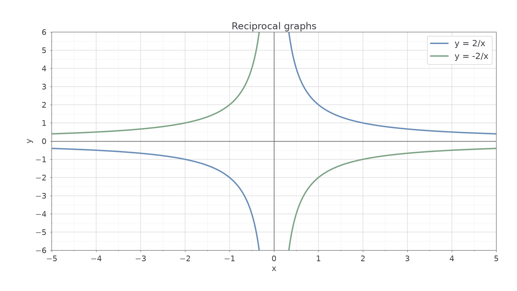
The asymptotes guide the shape; they are not extra graph segments. Never join a branch across the excluded input.

Worked example 3: plot two separate branches

Question. Make a table and draw $y=2/x$ on both sides of zero. State its excluded input and asymptotes.

Plan. Use positive and negative nonzero inputs, then draw each branch separately.

\begin{aligned} x=-0.5&:\quad y=\frac2{-0.5}=-4 &&\text{negative branch}\\ x=0.5&:\quad y=\frac2{0.5}=4 &&\text{positive branch} \end{aligned}

$x$	$-4$	$-2$	$-1$	$-0.5$	$0.5$	$1$	$2$	$4$
$y$	$-0.5$	$-1$	$-2$	$-4$	$4$	$2$	$1$	$0.5$

Why? No value exists at zero, so one continuous curve through the centre would add points that do not satisfy the equation.

Answer. Two smooth branches in quadrants I and III, as shown in blue. Exclude $x=0$ ; asymptotes $x=0$ and $y=0$ .

Check. Every table pair satisfies $xy=2$ , and no output is zero.

Change only the sign of the numerator next. Each output changes sign, so the branches move to the other two quadrants.

Worked example 4: a negative reciprocal

Question. Make a table and draw $y=-2/x$ , stating the excluded input and asymptotes.

Plan. Divide $-2$ by each input and keep the two branches separate.

\begin{aligned} x=-0.5&:\quad y=\frac{-2}{-0.5}=4 &&\text{negative input, positive output}\\ x=0.5&:\quad y=\frac{-2}{0.5}=-4 &&\text{positive input, negative output} \end{aligned}

$x$	$-4$	$-2$	$-1$	$-0.5$	$0.5$	$1$	$2$	$4$
$y$	$0.5$	$1$	$2$	$4$	$-4$	$-2$	$-1$	$-0.5$

Why? A negative numerator divided by a negative input is positive; divided by a positive input it is negative.

Answer. Two smooth branches in quadrants II and IV, shown in sage. Exclude $x=0$ ; the asymptotes remain $x=0$ and $y=0$ .

Check. Each pair satisfies $xy=-2$ , and the outputs are the negatives of example 3.

The domain is all nonzero real inputs. The range is all nonzero real outputs: approaching zero does not mean reaching it.

Watch out

The line $2/0=0$ is wrong: division by zero is undefined. Leave a break at $x=0$ ; do not insert the origin or connect the branches through it.

State an asymptote as a line equation, so its direction is clear.

Continue this lesson.

You’re previewing NovaLearn without an account. Create a free account to read the rest.

Create free account

Last Accessed

Number

Algebra

Shape, space and measure

Handling data

3.3 - Cubic and reciprocal graphs

Plotting cubic graphs (Higher)

Reciprocal graphs and asymptotes (Higher)

Continue this lesson.

Learn faster with Nova